soilVAE

Supervised Variational Autoencoder (VAE) regression for high‑dimensional predictors (e.g., VIS–NIR–SWIR soil spectroscopy), implemented in Python TensorFlow/Keras and exposed in R via reticulate.

The README is also the main reproducible case study, mirroring the vignette (vignettes/soilVAE-workflow.Rmd) so a reader can understand the why, how, and performance without opening additional files.

What soilVAE does

Given spectra \(x\in\mathbb{R}^p\) and a continuous soil property \(y\), soilVAE learns

• an encoder \(q_\phi(z\mid x)\) mapping spectra to a Gaussian latent \(z\in\mathbb{R}^d\),
• a decoder reconstructing \(x\) from a sample of \(z\),
• a regression head predicting \(y\) from the latent mean.

Objective

\[\mathcal{L} = \underbrace{\tfrac{1}{p}\|x-\hat x\|_2^2}_{\text{reconstruction}} \;+\; \beta\,\underbrace{D_{KL}\!\left(q_\phi(z\mid x)\,\|\,\mathcal{N}(0,I)\right)}_{\text{regularisation}} \;+\; \alpha\,\underbrace{(y_s-\hat y_s)^2}_{\text{regression}}\]

where \(y_s\) is \(y\) standardised by vae_fit(). The reconstruction error is averaged over the \(p\) predictors, so the three terms stay on comparable scales whatever the number of bands or the units of \(y\). In the API, beta_kl \(=\beta\) (default 1e-3) and alpha_y \(=\alpha\) (default 1). Predictions are deterministic and returned in the original units of \(y\).

Installation

install.packages("soilVAE")

soilVAE runs its model in Python (TensorFlow and Keras 3) through reticulate. Set the backend up once:

library(soilVAE)
vae_install()     # creates the "r-soilvae" virtualenv with TensorFlow and Keras
vae_available()   # TRUE when ready

soilVAE uses the "r-soilvae" environment automatically in later sessions. vae_available() only looks: it never installs or downloads anything.

Other setups:

• conda: vae_install(method = "conda").
• An existing environment with TensorFlow (>= 2.16) and Keras (>= 3): call vae_configure(venv = "name"), vae_configure(conda = "name") or vae_configure(python = "/path/to/python") at the start of each session.

reticulate binds one Python per R session. Choose the environment before calling any other soilVAE function; to switch, restart R.

Example: soil carbon from NIR spectra

The data are NIRsoil from the prospectr package, loaded from prospectr at run time. soilVAE contains code only and bundles no data.

library(soilVAE)
suppressPackageStartupMessages({library(prospectr); library(pls)})

data("NIRsoil", package = "prospectr")
d <- NIRsoil[is.finite(NIRsoil$Ciso), ]       # total carbon, %
cal <- d$train == 1                           # calibration / test split shipped with the data

# SNV; vae_fit() then centres and scales the bands with the calibration
# statistics and stores them, so vae_predict() scales new spectra the same way
X <- standardNormalVariate(d$spc)
X_cal <- X[cal, ];  y_cal <- d$Ciso[cal]
X_te  <- X[!cal, ]; y_te  <- d$Ciso[!cal]

metrics <- function(obs, pred) {
  rmse <- sqrt(mean((obs - pred)^2))
  c(R2 = 1 - sum((obs - pred)^2) / sum((obs - mean(obs))^2), RMSE = rmse, RPIQ = IQR(obs) / rmse)
}

PLS baseline, components chosen by 10-fold cross-validation:

set.seed(1)
pls_fit  <- plsr(y_cal ~ X_cal, ncomp = 30, validation = "CV")
ncomp    <- which.min(RMSEP(pls_fit)$val[1, 1, -1])
pls_pred <- predict(pls_fit, X_te, ncomp = ncomp)[, 1, 1]

soilVAE, with a fifth of the calibration set held out for early stopping:

set.seed(1)
va <- sample(nrow(X_cal), round(0.2 * nrow(X_cal)))

model <- vae_build(input_dim = ncol(X_cal), seed = 1L)
vae_fit(model, X_cal[-va, ], y_cal[-va], X_cal[va, ], y_cal[va],
        epochs = 300L, patience = 20L)
vae_pred <- vae_predict(model, X_te)

round(rbind(PLS = metrics(y_te, pls_pred), soilVAE = metrics(y_te, vae_pred)), 3)
#>            R2  RMSE  RPIQ
#> PLS     0.683 0.855 0.999
#> soilVAE 0.755 0.752 1.137

plot(y_te, vae_pred, xlab = "Observed carbon (%)", ylab = "Predicted carbon (%)",
     pch = 16, col = "grey30", main = "soilVAE, test set")
abline(0, 1, lty = 2)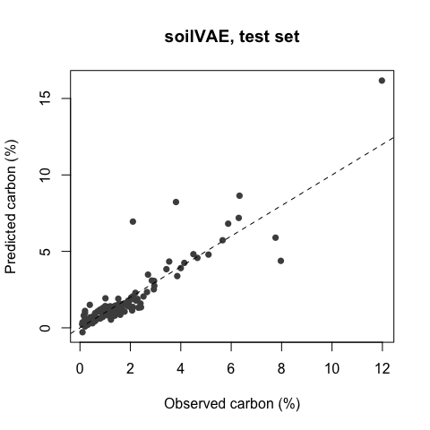

Other functions: vae_install() and vae_available() set up and check the Python backend, vae_encode() returns the latent embedding, vae_history() the training curves, vae_save() / vae_load() store a fitted model, and tune_vae_train_val() with select_best_from_grid() tune a grid of settings. See the vignette for a longer walk-through.

What changed in 0.2.0

Version 0.2.0 fixes defects that made 0.1.x predict poorly with its default settings (see NEWS.md): the reconstruction term was summed over all bands and swamped the regression term; early stopping watched the reconstruction rather than the prediction; the target was not standardised; a single hidden layer raised an error; models could not be saved; and tuning was not reproducible. Predictor and target scaling, column names and a “fitted” flag are now stored in the model, and every input is checked. With the defaults, the median test R² on NIRsoil is 0.78 over 10 seeds (PLS 0.68). The example dataset datsoilspc was removed: the package now contains code only.

Notes for life

Education without ethics is only rhetoric.

Power without reflection is violence