![]()
![]()
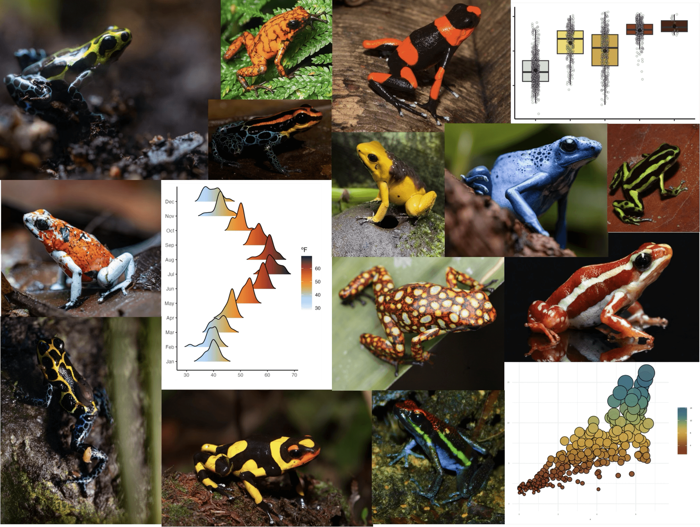
A collection of color palettes inspired by Neotropical poison frogs.
With more than 200 brighly colored species, Neotropical poison frogs
paint the rain forest in vivid hues that shout a clear message: “I’m
toxic!”. Spice up your plots with poisonfrogs and give your
dataviz a toxic twist! But wait, we also included some color palettes
inspired by other pretty frog species, because… why not? 🐸
Get inspired with the collection of species behind the color palettes.
You can install poisonfrogs from CRAN:
install.packages("poisonfrogs")or from the development version in GitHub with:
remotes::install_github("laurenoconnelllab/poisonfrogs")load the package:
library(poisonfrogs)poisonfrogs
color palettes “At a glance”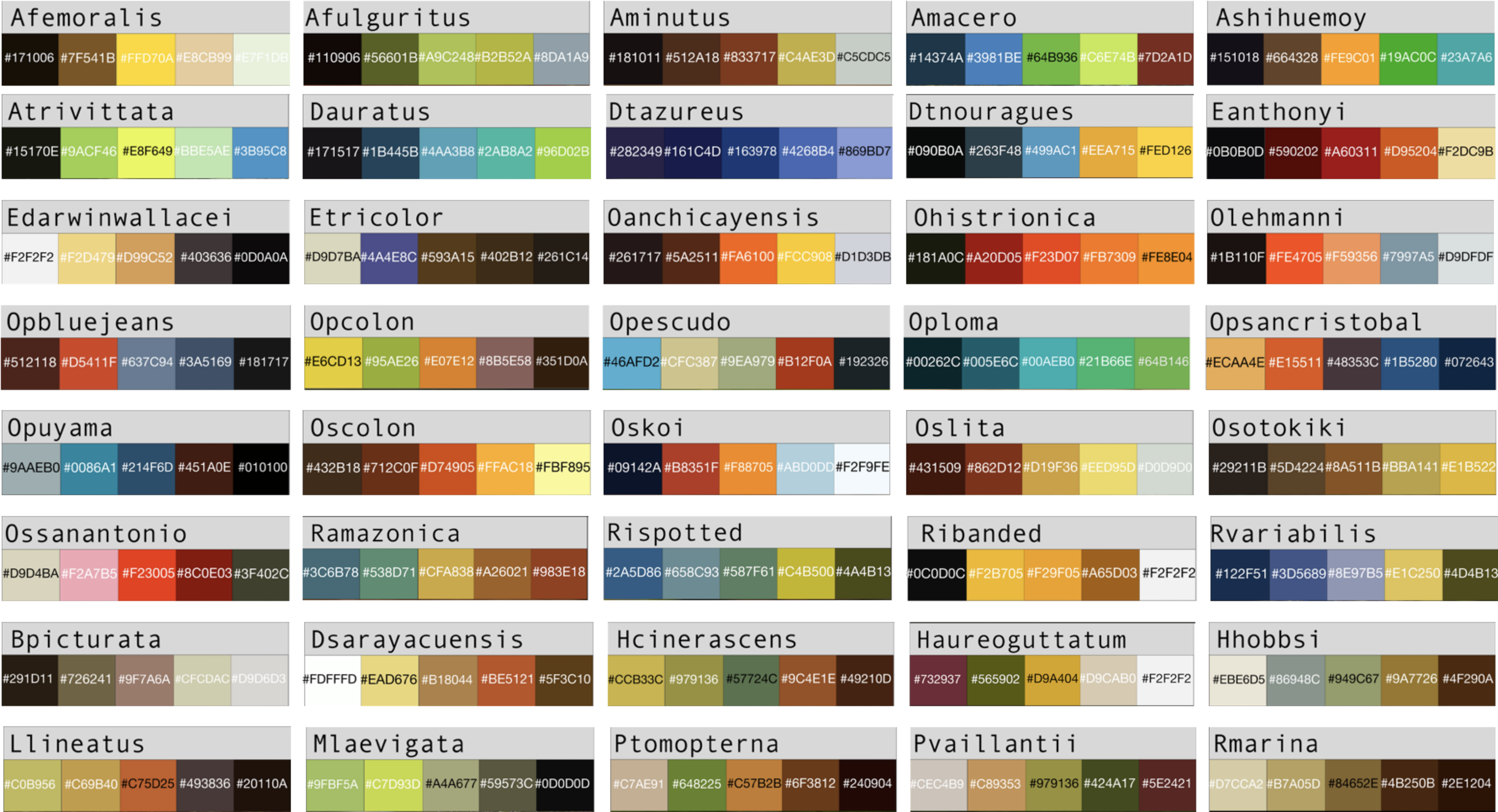
To see the names of all colour palettes in poisonfrogs:
poison_palettes_names()
#>  [1] "Afemoralis"      "Afulguritus"     "Amacero"         "Aminutus"
#>  [5] "Ashihuemoy"      "Atrivittata"     "Bpicturata"      "Dauratus"
#>  [9] "Dsarayacuensis"  "Dtazureus"       "Dtnouragues"     "Eanthonyi"
#> [13] "Edarwinwallacei" "Etricolor"       "Haureoguttatum"  "Hcinerascens"
#> [17] "Hhobbsi"         "Llineatus"       "Mlaevigata"      "Oanchicayensis"
#> [21] "Ohistrionica"    "Olehmanni"       "Opbluejeans"     "Opcolon"
#> [25] "Opescudo"        "Oploma"          "Opsancristobal"  "Opuyama"
#> [29] "Oscolon"         "Oskoi"           "Oslita"          "Osotokiki"
#> [33] "Ossanantonio"    "Pterribilis"     "Ptomopterna"     "Pvaillantii"
#> [37] "Ramazonica"      "Ribanded"        "Rispotted"       "Rmarina"
#> [41] "Rvariabilis"
Visualize poison frog palettes:
poison_palette("Haureoguttatum")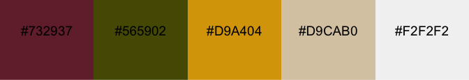
or get their hex codes:
poison_palette("Haureoguttatum", return = "vector")
#> [1] "#732937" "#565902" "#D9A404" "#D9CAB0" "#F2F2F2"poisonfrogs in base R plots
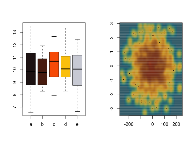
par(mfrow = c(1, 2))

#Discrete scale

group <- factor(sample(letters[1:5], 100, replace = TRUE))

value <- rnorm(100, mean = 10, sd = 1.5)

boxplot(value ~ group,
        col = poison_palette(
    "Oanchicayensis",
    return = "vector",
    type = "discrete",
    direction = 1
  ),
  xlab = "",
  ylab = "")

#Continuous scale
x <- rnorm(1000) * 77
y <- rnorm(1000)

smoothScatter(
  y ~ x,
  colramp = colorRampPalette(poison_palette(
    "Ramazonica",
    return = "vector",
    type = "continuous",
    direction = 1
  )),
  xlab = "",
  ylab = ""
)
poison scales in ggplot2scale_fill_poison()
require(tidyverse)
require(gapminder)
require(ggridges)
require(scales)
require(patchwork)

#continuous scale

df_nottem <- tibble(
  year  = floor(time(nottem)),
  month = factor(month.abb[cycle(nottem)], levels = month.abb),
  temp  = as.numeric(nottem)
)

p1 <- ggplot(df_nottem, aes(x = temp, y = month, fill = after_stat(x))) +
  geom_density_ridges_gradient(scale = 2, rel_min_height = 0.01) +
  scale_fill_poison(
    name = "Oskoi",
    type = "continuous",
    alpha = 0.95,
    direction = -1) +
  labs(
  fill = "ºF",
  y = NULL,
  x = NULL) +
  theme_classic(base_size = 10, base_line_size = 0.5) +
  theme(legend.position = "right", legend.justification = "left",
  legend.margin = margin(0,0,0,0),
  legend.box.margin = margin(-5,-5,-5,-5)) +
  coord_cartesian(clip = "off")


#discrete scale
p2 <- ggplot(gapminder, aes(x = continent, y = lifeExp, fill = continent)) +
  geom_boxplot(outliers = F) +
  geom_jitter(
    shape = 21,
    position = position_jitter(0.1),
    alpha = 0.2,
    size = 0.8,
    bg = "grey"
  ) +
  stat_summary(
    fun = mean,
    geom = "point",
    size = 1.5,
    color = "black",
    alpha = 0.6
  ) +
  #theme_classic(base_size = 20, base_line_size = 0.5) +
  scale_fill_poison(
    name = "Amacero",
    type = "discrete",
    alpha = 0.9,
    direction = 1
  ) +
  theme(legend.position = "none") +
  xlab(NULL) +
  ylab("Life Expentancy")

p1 + p2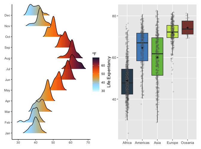
scale_color_poison()
#Continuous scale

set.seed(42)
n <- 300
x <- runif(n, 0, 10)
y <- 1.5 + 0.9 * x + rnorm(n, sd = 0.4 + 0.25 * x)
sz <- rescale(y, to = c(2, 14))

df <- data.frame(x, y, sz)

p3 <- ggplot(df, aes(x, y)) +
  geom_point(
    aes(color = y, size = sz),
    shape = 16,
    alpha = 0.95,
    stroke = 0.6
  ) +
  scale_size_identity(guide = "none") +
  scale_color_poison("Ramazonica", type = "continuous", direction = 1) +
  theme_minimal() +
  ylim(0, 18) +
  xlim(0, 11)


#discrete scale
p4 <- ggplot(gapminder, aes(x = lifeExp, y = log(gdpPercap), colour = continent)) +
  geom_point(alpha = 0.4) +
  scale_colour_poison(name = "Opcolon", type = "discrete") +
  stat_smooth() +
  facet_wrap(.~continent, scales = "free") +
  theme_minimal(10, base_line_size = 0.2) +
  theme(legend.position = "none",
  strip.background = element_blank(), strip.placement = "outside")

p3 + p4 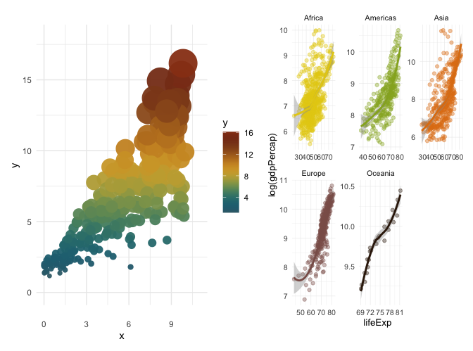
Need a high-speed mirror for your open-source project?
Contact our mirror admin team at info@clientvps.com.
This archive is provided as a free public service to the community.
Proudly supported by infrastructure from VPSPulse , RxServers , BuyNumber , UnitVPS , OffshoreName and secure payment technology by ArionPay.