ivue is an R package for interactive three-dimensional visualization of data and embedded graphs. Combine point clouds and graph edges with numerical or categorical colors, labels, paths, and surfaces; explore them in RStudio or a web browser; and share them as interactive HTML. Reusable color scales and camera controls keep related views consistent, while coordinate animations let you follow a changing shape or recorded layout. ivue works with coordinates from your chosen analysis or embedding method.
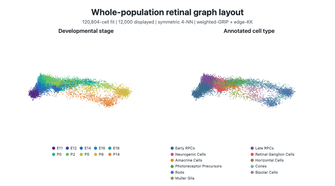
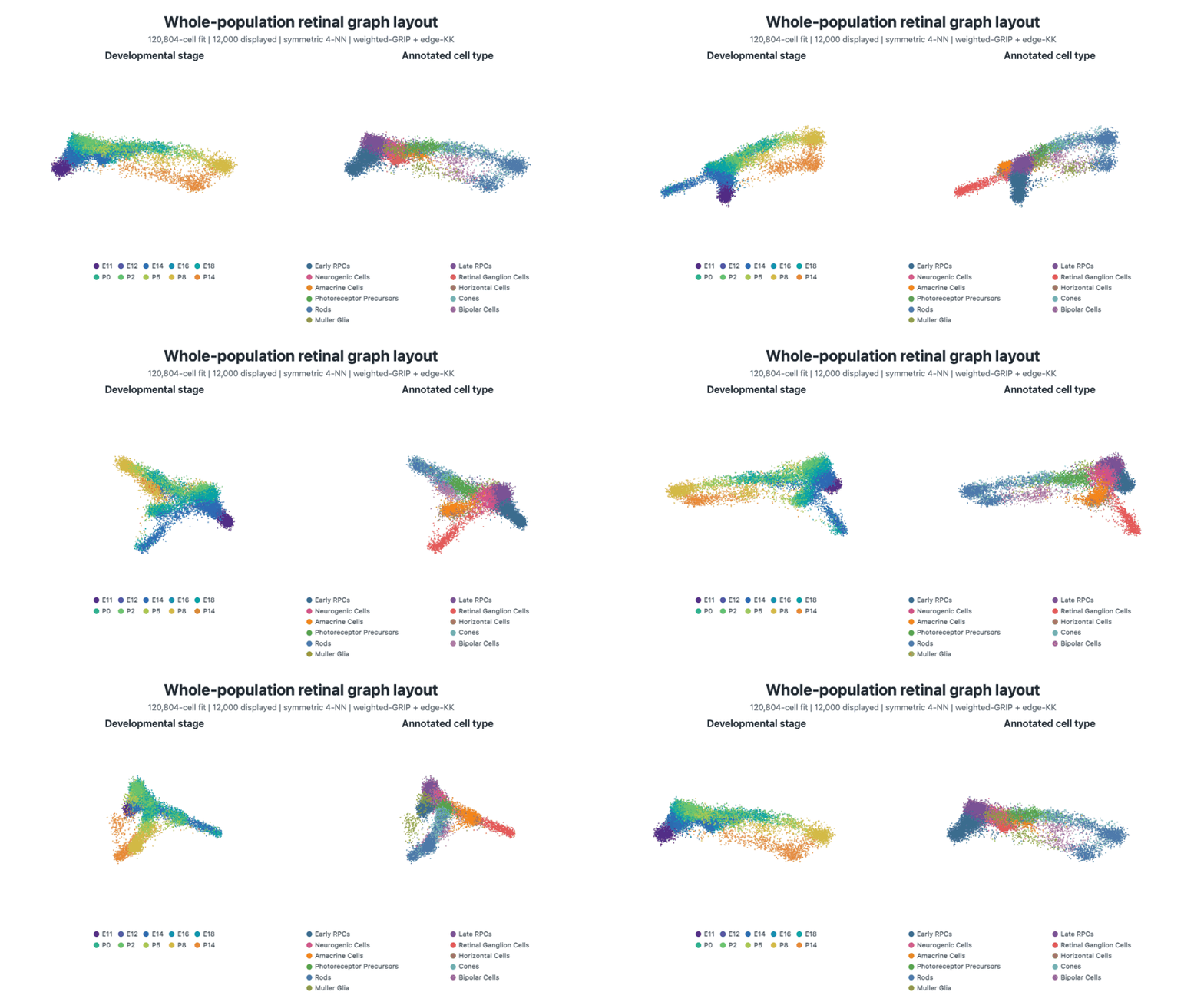
The following animation shows the same 12,000 mouse retinal cells
colored by developmental stage and annotated cell type. Shared
coordinates and synchronized views show how the two annotations relate.
The data come from Clark et
al. (2019); the layout was computed with dgraphs and
grip, then rendered with ivue. The retinal-development
vignette presents the complete example and its provenance, while the
introduction
vignette explains the plotting controls.
View a static alternative without motion.
Install the current development build (not yet a CRAN release). This built source package includes all five rendered guides. Install its dependencies first:
install.packages(c("htmlwidgets", "htmltools", "rgl"))
install.packages("https://pgajer.github.io/ivue/ivue_0.1.0.tar.gz",
                 repos = NULL, type = "source")
vignette("function-guide", package = "ivue")
The documentation site
identifies the source commit and provides the same guides online. The
built package includes them for offline reading; you do not need
knitr, rmarkdown, or Pandoc to read them.
Start with a coordinate matrix, one observation per row. This sample from a saddle is colored by height:
library(ivue)
set.seed(1)
x <- runif(250, -1, 1)
y <- runif(250, -1, 1)
X <- cbind(x = x, y = y, z = 1.2 * (x^2 - y^2))
plot3D.cont(X, values = X[, "z"], legend.title = "Saddle height")
The plot opens in RStudio’s Viewer or your browser, where you can
rotate and zoom it. No native graphics window or XQuartz setup is
needed. Assign the returned widget to a variable to reuse it or save it
with htmlwidgets::saveWidget().
With explicit coordinate row IDs, named annotations match those IDs in both point-cloud and graph views. Unnamed annotations follow row order. See the input recipes for checks and a shuffled-annotation example.
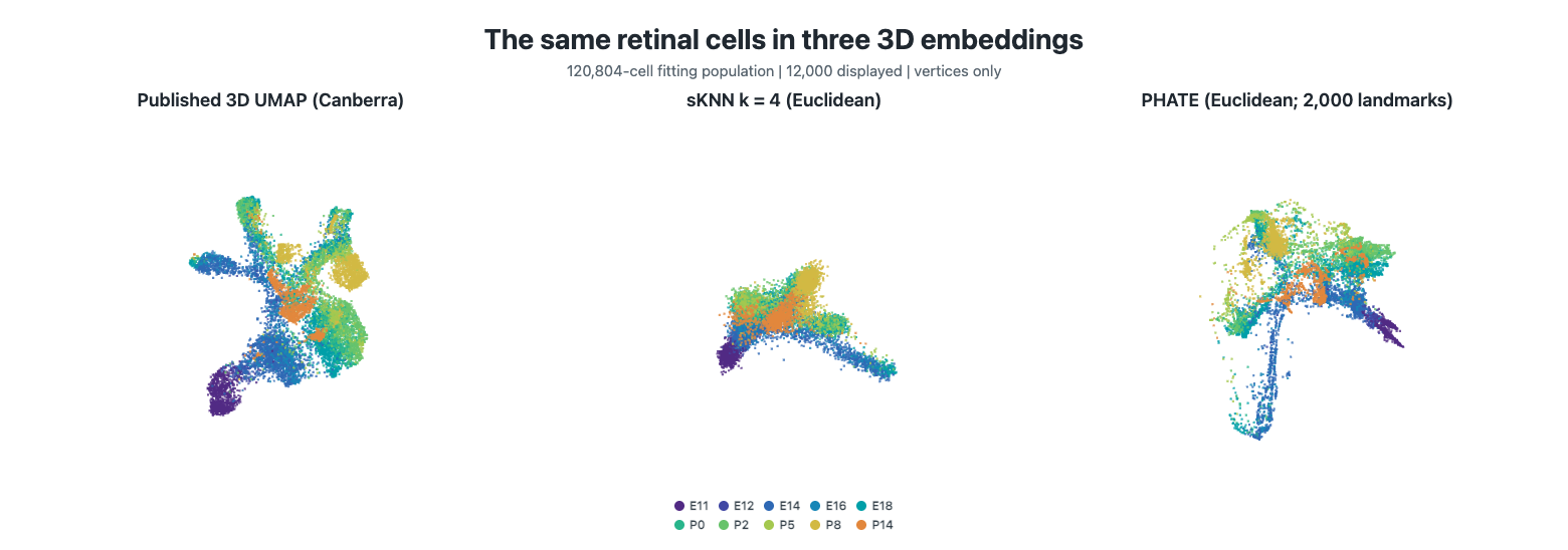
The same plotting controls also let you compare coordinate systems while keeping observations and colors fixed. Below, the retinal cells appear in published UMAP coordinates, a symmetric-kNN graph layout fitted with weighted-GRIP followed by edge-KK refinement, and a PHATE embedding.
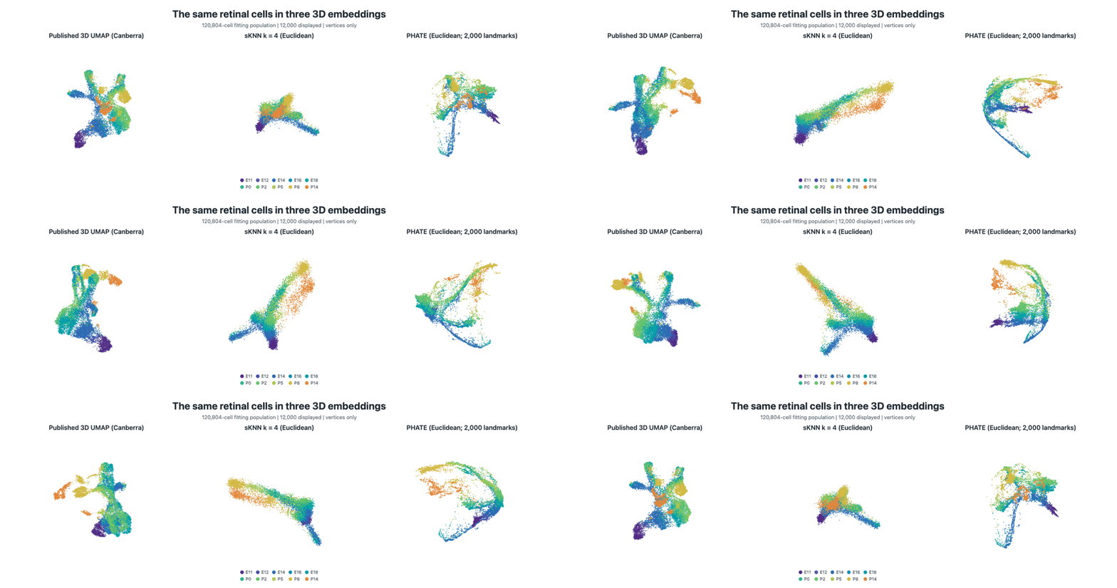
View a static alternative without motion.
All three embeddings were fitted on 120,804 cells before selecting the same 12,000 retained retinal cells for display. UMAP uses Canberra distance; the symmetric 4-nearest-neighbor graph and PHATE use Euclidean distance. PHATE uses 2,000 spectral landmarks and an automatically selected diffusion time. All panels show points without edges and complete a rotation in 14.4 seconds, starting with their P14 centroids facing the viewer. ivue renders the supplied coordinates without computing the embeddings.
The vignettes develop these examples and show how to adapt them to your data:
The links above open rendered guides. Their maintained sources are on GitHub. Open the same guides from your installation with:
vignette("function-guide", package = "ivue")
vignette("example-data", package = "ivue")
vignette("ivue-introduction", package = "ivue")
vignette("retinal-development", package = "ivue")
vignette("animation", package = "ivue")
Report problems or suggest improvements in the issue tracker.