
Events from individual hydrologic time series are extracted, and events from multiple time series can be matched to each other.
This code can be downloaded from CRAN: https://cran.r-project.org/package=hydroEvents
A detailed description of each function, usage, and suggested parameters is provided in the following: Wasko, C., Guo, D., 2022. Understanding event runoff coefficient variability across Australia using the hydroEvents R package. Hydrol. Process. 36, e14563. https://doi.org/10.1002/hyp.14563
If using this code a citation to the above manuscript would be greatly appreciated.
Aim: Calculate baseflow and baseflow index
This code reproduces Figure 5 in Wasko and Guo (2022).
library(hydroEvents)
bf.A.925 = baseflowA(dataBassRiver, alpha = 0.925)$bf
bf.A.980 = baseflowA(dataBassRiver, alpha = 0.980)$bf

bf.B.925 = baseflowB(dataBassRiver, alpha = 0.925)$bf
bf.B.980 = baseflowB(dataBassRiver, alpha = 0.980)$bf

bfi.A.925 = sum(bf.A.925)/sum(dataBassRiver) # 0.22
bfi.A.980 = sum(bf.A.980)/sum(dataBassRiver) # 0.09
bfi.B.925 = sum(bf.B.925)/sum(dataBassRiver) # 0.39
bfi.B.980 = sum(bf.B.980)/sum(dataBassRiver) # 0.20

plot(dataBassRiver, type = "l", col = "#377EB8", lwd = 2, mgp = c(2, 0.6, 0), ylab = "Flow (ML/day)", xlab = "Index", xlim = c(0, 70))
lines(bf.A.925, lty = 2)
lines(bf.A.980, lty = 3)
lines(bf.B.925, lty = 1)
lines(bf.B.980, lty = 4)
legend("topright", lty = c(2, 3, 1, 4), col = c("black", "black", "black", "black"), cex = 0.8, bty = "n",
       legend = c(paste0("BFI(A, 0.925) = ", format(round(bfi.A.925, 2), nsmall = 2)),
                  paste0("BFI(A, 0.980) = ", format(round(bfi.A.980, 2), nsmall = 2)),
                  paste0("BFI(B, 0.925) = ", format(round(bfi.B.925, 2), nsmall = 2)),
                  paste0("BFI(B, 0.980) = ", format(round(bfi.B.980, 2), nsmall = 2))))
Aim: Extract precipitation events
events = eventPOT(dataLoch, threshold = 1, min.diff = 2)
plotEvents(dataLoch, dates = NULL, events = events, type = "hyet", ylab = "Rainfall [mm]", main = "Rainfall Events (threshold = 1, min.diff = 2)")
Aim: Extract flow events (and demonstrate the different methods available)
This code reproduces Figure 6 in Wasko and Guo (2022).
library(hydroEvents)
bf = baseflowB(dataBassRiver)
Max_res = eventMaxima(dataBassRiver-bf$bf, delta.y = -0.75, delta.x = 1, threshold = 0)
Min_res = eventMinima(dataBassRiver-bf$bf, delta.y = 100, delta.x = 3, threshold = 0)
PoT_res = eventPOT(dataBassRiver-bf$bf, threshold = 0, min.diff = 1)
BFI_res = eventBaseflow(dataBassRiver, BFI_Th = 0.5, min.length = 1)

par(mfrow = c(2, 2), mar = c(3, 2.7, 2, 1))
plotEvents(data = dataBassRiver, events = PoT_res, ymax = 1160, xlab = "Index", ylab = "Flow (ML/day)", colpnt = "#E41A1C", colline = "#377EB8", main = "eventPOT")
lines(1:length(bf$bf), bf$bf, lty = 2)
plotEvents(data = dataBassRiver, events = Max_res, ymax = 1160, xlab = "Index", ylab = "Flow (ML/day)", colpnt = "#E41A1C", colline = "#377EB8", main = "eventMaxima")
lines(1:length(bf$bf), bf$bf, lty = 2)
plotEvents(data = dataBassRiver, events = Min_res, ymax = 1160, xlab = "Index", ylab = "Flow (ML/day)", colpnt = "#E41A1C", colline = "#377EB8", main = "eventMinima")
lines(1:length(bf$bf), bf$bf, lty = 2)
plotEvents(data = dataBassRiver, events = BFI_res, ymax = 1160, xlab = "Index", ylab = "Flow (ML/day)", colpnt = "#E41A1C", colline = "#377EB8", main = "eventBaseflow")
lines(1:length(bf$bf), bf$bf, lty = 2)
Aim: Identify rising and falling limbs
library(hydroEvents)
qdata = WQ_Q$qdata[[1]]
BF_res = eventBaseflow(qdata$Q_cumecs)
limbs(data = qdata$Q_cumecs, dates = NULL, events = BF_res, main = "with 'eventBaseflow'")
Aim: Calculate CQ (concentration-discharge) relationships
library(hydroEvents)
# Identify flow events
qdata = WQ_Q$qdata[[1]]
BF_res = eventBaseflow(qdata$Q_cumecs)
MAX_res = eventMaxima(qdata$Q_cumecs, delta.y = 0.5, threshold = 0.5)

# Aggregate water quality data to daily time step
wqdata=WQ_Q$wqdata[[1]]
wqdata = data.frame(time=wqdata$time,wq=as.vector(wqdata$WQ))

wqdaily = rep(NA,length(unique(substr(wqdata$time,1,10))))
for (i in 1:length(unique(substr(wqdata$time,1,10)))) {
  wqdaily[i] = mean(wqdata$wq[which(substr(wqdata$time,1,10)==
                                      unique(substr(wqdata$time,1,10))[i])])
}
wqdailydata = data.frame(time=as.Date(strptime(unique(substr(wqdata$time,1,10)),"%d/%m/%Y")),wq=wqdaily)

# A function to plot the CQ relationship by event period
CQ_event = function(C,Q,events,methodname) {
  QinWQ = which(Q$time%in%C$time)

  risfal_res = limbs(data=as.vector(Q$Q_cumecs),events=events,main = paste("Events identified -",methodname))

  allRL_ind = unlist(apply(risfal_res,1,function(x){x[6]:x[7]}))
  allFL_ind = unlist(apply(risfal_res,1,function(x){x[8]:x[9]}))

  RL_ind = which(allRL_ind%in%QinWQ)
  FL_ind = which(allFL_ind%in%QinWQ)

  allEV_ind = unlist(apply(risfal_res,1,function(x){x[1]:x[2]}))
  allBF_ind = as.vector(1:length(as.vector(Q$Q_cumecs)))[-allEV_ind]
  EV_ind = which(allEV_ind%in%QinWQ)
  BF_ind = which(allBF_ind%in%QinWQ)

  RL_indwq = which(QinWQ%in%allRL_ind[RL_ind])
  FL_indwq = which(QinWQ%in%allFL_ind[FL_ind])
  BF_indwq = which(QinWQ%in%allBF_ind[BF_ind])
  EV_indwq = which(QinWQ%in%allEV_ind[EV_ind])

  plot(C$wq~Q$Q_cumecs[QinWQ],xlab="Q (mm/d)",ylab="C (mg/L)",main = paste("C-Q relationship -",methodname),pch=20)
  points(C$wq[RL_indwq]~Q$Q_cumecs[allRL_ind[RL_ind]],col="blue",pch=20)
  points(C$wq[FL_indwq]~Q$Q_cumecs[allFL_ind[FL_ind]],col="red",pch=20)
  points(C$wq[BF_indwq]~Q$Q_cumecs[allBF_ind[BF_ind]],col="grey",pch=20)

  legend("topright",
         legend=c("rising limb","falling limb","baseflow"),
         pch=20,col=c("blue","red","grey"))

  CQ = cbind(C$wq,Q$Q_cumecs[QinWQ])
  res = list(event=EV_indwq,base=BF_indwq,rising=RL_indwq,falling=FL_indwq,
             eventCQ=CQ[EV_indwq,],baseCQ=CQ[BF_indwq,],
             risingCQ=CQ[RL_indwq,],fallingCQ=CQ[FL_indwq,])
}

# Final plot of CQ comparison from two event approaches
par(mfcol=c(2,2))
par(mar=c(2,2,2,2))
CQ_event(wqdailydata,qdata, BF_res, methodname="eventBaseflow")
CQ_event(wqdailydata,qdata, MAX_res, methodname="eventMaxima")Aim: Demonstrate matching rainfall to runoff
library(hydroEvents)
# Prepare data
srt = as.Date("2015-02-05")
end = as.Date("2015-04-01")
dat = dataCatchment$`105105A`[which(dataCatchment$`105105A`$Date >= srt & dataCatchment$`105105A`$Date <= end),]

# Extract events
events.P = eventPOT(dat$Precip_mm, threshold = 1, min.diff = 1)
events.Q = eventMaxima(dat$Flow_ML, delta.y = 2, delta.x = 1, thresh = 70)

par(mfrow = c(2, 1), mar = c(3, 2.7, 2, 1))
plotEvents(dat$Precip_mm, dates = dat$Date, events = events.P, type = "hyet", colline = "#377EB8", colpnt = "#E41A1C",ylab = "Rainfall (mm)", xlab = 2015, main = "")
plotEvents(dat$Flow_ML,   dates = dat$Date, events = events.Q, type = "lineover", colpnt = "#E41A1C", colline = "#377EB8", ylab = "Flow (ML/day)", xlab = 2015, main = "")
The following code reproduces Figure 7 in Wasko and Guo (2022).
# Match events
library(RColorBrewer)
matched.1 = pairEvents(events.P, events.Q, lag = 5,  type = 1)
matched.2 = pairEvents(events.P, events.Q, lag = 5,  type = 2)
matched.3 = pairEvents(events.P, events.Q, lag = 3,  type = 3)
matched.4 = pairEvents(events.P, events.Q, lag = 7, type = 4)
matched.5 = pairEvents(events.P, events.Q, lag = 5, type = 5)

par(mfrow = c(3, 2), mar = c(1.7, 3, 2.1, 3))
plotPairs(data.1 = dat$Precip_mm, data.2 = dat$Flow_ML, events = matched.1, date = dat$Date, col = brewer.pal(nrow(events.P), "Set3"), main = "Type 1", ylab.1 = "Rainfall (mm)", ylab.2 = "Flow (ML/day)", cex.2 = 2/3)
plotPairs(data.1 = dat$Precip_mm, data.2 = dat$Flow_ML, events = matched.2, date = dat$Date, col = brewer.pal(nrow(events.P), "Set3"), main = "Type 2", ylab.1 = "Rainfall (mm)", ylab.2 = "Flow (ML/day)", cex.2 = 2/3)
plotPairs(data.1 = dat$Precip_mm, data.2 = dat$Flow_ML, events = matched.3, date = dat$Date, col = brewer.pal(nrow(events.P), "Set3"), main = "Type 3", ylab.2 = "Rainfall (mm)", ylab.1 = "Flow (ML/day)", cex.2 = 2/3)
plotPairs(data.1 = dat$Precip_mm, data.2 = dat$Flow_ML, events = matched.4, date = dat$Date, col = brewer.pal(nrow(events.P), "Set3"), main = "Type 4", ylab.2 = "Rainfall (mm)", ylab.1 = "Flow (ML/day)", cex.2 = 2/3)
plotPairs(data.1 = dat$Precip_mm, data.2 = dat$Flow_ML, events = matched.5, date = dat$Date, col = brewer.pal(nrow(events.P), "Set3"), main = "Type 5", ylab.1 = "Rainfall (mm)", ylab.2 = "Flow (ML/day)", cex.2 = 2/3) 
Aim: Demonstrate matching of rainfall and water level surge (residuals)
library(hydroEvents)

# Hourly rainfall (P) and water level surge (WL) at Burnie, Tasmania (Pluvio 91009; Tide gauge: IDO71005)
Psel  = data_P_WL$Psel
WLsel = data_P_WL$WLsel

# Find events in P and WL data
# Rain over 4mm is considered an event; events over 3 hrs apart are considered as separate
events.P = eventPOT(Psel, threshold = 4, min.diff = 3)

# WL surge residual over 0.05m is considered an event; events over 3 hrs apart are considered as separate
events.Q1 = eventMaxima(WLsel, delta.y = 0.05, delta.x = 3, thresh = 0.05)

# Plot events
plotEvents(data = Psel, events = events.P, main = "Hourly precipitation (mm)", type = "hyet")
plotEvents(data = WLsel, events = events.Q1, main = "Hourly water level surge (m)", type = "lineover")
# Pairing events - use type = 5 to search both ways for the pairing
# Try two different values for the lag (search radius)
matched.1 = pairEvents(events.P, events.Q1, lag = 12, type = 5)
matched.2 = pairEvents(events.P, events.Q1, lag = 24, type = 5)

plotPairs(data.1 = Psel, data.2 = WLsel, events = matched.1, type = "hyet", color.list=rainbow(nrow(matched.1)))
plotPairs(data.1 = Psel, data.2 = WLsel, events = matched.2, type = "hyet", color.list=rainbow(nrow(matched.2)))
Aim: Demonstrate event identification with hourly streamflow data
library(hydroEvents)
library(stats)
# Prepare data
data(hourlyQ)

# smoothing for hourly data to remove local fluctuation
flow = hourlyQ$q
n = length(flow)
flow.smoothed = filter(flow, c(0.1, 0.2, 0.4, 0.2, 0.1))[3:(n-2)]

# baseflow filtering and event identification with eventMaxima
bf = baseflowA(flow.smoothed, alpha = 0.925)
events = eventMaxima(flow.smoothed-bf$bf, -0.75, 12, threshold = 1)
idx = 63800
events$srt = events$srt - idx
events$end = events$end - idx
plotEvents(data = flow[3:(n-2)][idx:(idx+200)], events = events[120,], type = "lineover", xlab = "Index", ylab = "Flow (m3/s)", colpnt = "#E41A1C", colline = "#377EB8", main = "Event Identification with Hourly Data")
lines(1:201, bf$bf[idx:(idx+200)], lty = 2)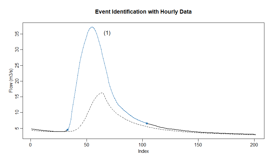
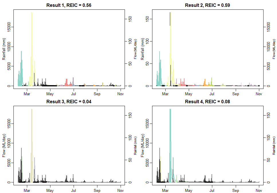
Aim: Demonstrate the calculation of the Robust Event Identification Criteria (REIC), following Mohammadpour Khoie, et al. (2025): https://doi.org/10.1016/j.envsoft.2025.106521. Calculation of the REIC value for a set of rainfall-runoff events given rainfall and runoff time series and events
library(RColorBrewer)
dat = dataCatchment$`105105A`
srt = as.Date("2015-02-05")
end = as.Date("2015-11-01")
dat = dataCatchment$`105105A`[which(dataCatchment$`105105A`$Date >= srt & dataCatchment$`105105A`$Date <= end),]


events.P = eventPOT(dat$Precip_mm, threshold = 1, min.diff = 1)
QF <- dat$Flow_ML-baseflowA(dat$Flow_ML, alpha = 0.925, passes = 3)$bf
events.Qbest1 = eventMinima(QF, delta.y = 14.24, delta.x = 1, thresh = 6.58)
matched.best1 = PostCorrection(pairEvents(events.P, events.Qbest1, lag = 6,  type = 3))

events.Qbest2 = eventMinima(QF, delta.y = 21.37, delta.x = 5, thresh = 2.42)
matched.best2 = PostCorrection(pairEvents(events.P, events.Qbest1, lag = 7,  type = 5))

events.Qworst1 = eventMaxima(QF, delta.y = -0.861, delta.x = 1, thresh = 127.1)
matched.worst1 = PostCorrection(pairEvents(events.P, events.Qworst1, lag = 1,  type = 4))

events.Qworst2 = eventMaxima(QF, delta.y = -0.825, delta.x = 9, thresh = 39.26)
matched.worst2 = PostCorrection(pairEvents(events.P, events.Qworst2, lag = 1,  type = 4))

REIC.b1 <- round(calcREIC(dat$Precip_mm, dat$Flow_ML, matched.best1, n_rainfall = nrow(events.P), area = 297),2) # see manual 'dataCatchment'
REIC.b2 <- round(calcREIC(dat$Precip_mm, dat$Flow_ML, matched.best2, n_rainfall = nrow(events.P), area = 297),2) # see manual 'dataCatchment'

REIC.w1 <- round(calcREIC(dat$Precip_mm, dat$Flow_ML, matched.worst1, n_rainfall = nrow(events.P), area = 297),2) # see manual 'dataCatchment'
REIC.w2 <- round(calcREIC(dat$Precip_mm, dat$Flow_ML, matched.worst2, n_rainfall = nrow(events.P), area = 297),2) # see manual 'dataCatchment'

par(mfrow = c(2, 2), mar = c(1.7, 3, 2.1, 3))
plotPairs(data.1 = dat$Precip_mm, data.2 = dat$Flow_ML, events = matched.best1, date = dat$Date, col = colorRampPalette(brewer.pal(12, "Set3"))(nrow(events.P)),
          main = paste("Result 1, REIC =",REIC.b1), ylab.1 = "Rainfall (mm)", ylab.2 = "Flow (ML/day)", cex.2 = 2/3)
plotPairs(data.1 = dat$Precip_mm, data.2 = dat$Flow_ML, events = matched.best2, date = dat$Date, col = colorRampPalette(brewer.pal(12, "Set3"))(nrow(events.P)),
          main = paste("Result 2, REIC =",REIC.b2), ylab.1 = "Rainfall (mm)", ylab.2 = "Flow (ML/day)", cex.2 = 2/3)
plotPairs(data.1 = dat$Precip_mm, data.2 = dat$Flow_ML, events = matched.worst1, date = dat$Date, col = colorRampPalette(brewer.pal(12, "Set3"))(nrow(events.P)),
          main = paste("Result 3, REIC =",REIC.w1), ylab.2 = "Rainfall (mm)", ylab.1 = "Flow (ML/day)", cex.2 = 2/3)
plotPairs(data.1 = dat$Precip_mm, data.2 = dat$Flow_ML, events = matched.worst2, date = dat$Date, col = colorRampPalette(brewer.pal(12, "Set3"))(nrow(events.P)),
          main = paste("Result 4, REIC =",REIC.w2), ylab.2 = "Rainfall (mm)", ylab.1 = "Flow (ML/day)", cex.2 = 2/3)
Need a high-speed mirror for your open-source project?
Contact our mirror admin team at info@clientvps.com.
This archive is provided as a free public service to the community.
Proudly supported by infrastructure from VPSPulse , RxServers , BuyNumber , UnitVPS , OffshoreName and secure payment technology by ArionPay.