![]()
![]()
The goal of healthyR is to help quickly analyze common data problems in the Administrative and Clincial spaces.
You can install the released version of healthyR from CRAN with:
install.packages("healthyR")And the development version from GitHub with:
# install.packages("devtools")
devtools::install_github("spsanderson/healthyR")This is a basic example of using the ts_median_excess_plt() function`:
library(healthyR)
library(timetk)
library(dplyr)

ts_signature_tbl(.data = m4_daily, .date_col = date, .pad_time = TRUE, id) %>%
    ts_median_excess_plt(
        .date_col           = date
        , .value_col        = value
        , .x_axis           = week
        , .ggplot_group_var = year
        , .years_back       = 5
    )
Here is a simple example of using the ts_signature_tbl() function:
library(healthyR)
library(timetk)
ts_signature_tbl(.data = m4_daily, .date_col = date)
#> # A tibble: 17,578 × 31
#> id date value index.num diff year year.iso half quarter month
#> <fct> <date> <dbl> <dbl> <dbl> <int> <int> <int> <int> <int>
#> 1 D410 1978-06-23 9109. 267408000 NA 1978 1978 1 2 6
#> 2 D410 1978-06-24 9103. 267494400 86400 1978 1978 1 2 6
#> 3 D410 1978-06-25 9116. 267580800 86400 1978 1978 1 2 6
#> 4 D410 1978-06-26 9116. 267667200 86400 1978 1978 1 2 6
#> 5 D410 1978-06-27 9106. 267753600 86400 1978 1978 1 2 6
#> 6 D410 1978-06-28 9094. 267840000 86400 1978 1978 1 2 6
#> 7 D410 1978-06-29 9094. 267926400 86400 1978 1978 1 2 6
#> 8 D410 1978-06-30 9084. 268012800 86400 1978 1978 1 2 6
#> 9 D410 1978-07-01 9081. 268099200 86400 1978 1978 2 3 7
#> 10 D410 1978-07-02 9047. 268185600 86400 1978 1978 2 3 7
#> # ℹ 17,568 more rows
#> # ℹ 21 more variables: month.xts <int>, month.lbl <ord>, day <int>, hour <int>,
#> # minute <int>, second <int>, hour12 <int>, am.pm <int>, wday <int>,
#> # wday.xts <int>, wday.lbl <ord>, mday <int>, qday <int>, yday <int>,
#> # mweek <int>, week <int>, week.iso <int>, week2 <int>, week3 <int>,
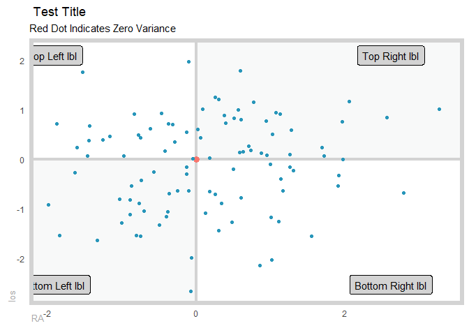
#> # week4 <int>, mday7 <int>Here is a simple example of using the plt_gartner_magic_chart() function:
suppressPackageStartupMessages(library(healthyR))
suppressPackageStartupMessages(library(tibble))
suppressPackageStartupMessages(library(dplyr))

gartner_magic_chart_plt(
  .data = tibble(x = rnorm(100, 0, 1), y = rnorm(100, 0, 1))
  , .x_col = x
  , .y_col = y
  , .y_lab = "los"
  , .x_lab = "RA"
  , .plot_title = "Test Title"
  , .top_left_label = "Top Left lbl"
  , .top_right_label = "Top Right lbl"
  , .bottom_left_label = "Bottom Left lbl"
  , .bottom_right_label = "Bottom Right lbl"
)
Need a high-speed mirror for your open-source project?
Contact our mirror admin team at info@clientvps.com.
This archive is provided as a free public service to the community.
Proudly supported by infrastructure from VPSPulse , RxServers , BuyNumber , UnitVPS , OffshoreName and secure payment technology by ArionPay.