README

grip embeds graphs in Euclidean space and helps assess how well the resulting coordinates preserve graph distances and local structure.

Start with metric multidimensional scaling (MDS) using stochastic gradient descent (SGD). Use full metric MDS when pairwise graph distances are affordable, and sparse metric MDS for larger problems. Targets can be unweighted hop distances or shortest-path distances defined by positive edge lengths.

The package also provides classical MDS, multiscale GRIP layouts, alternative optimization methods, and tools for comparing and visualizing embeddings. Use 2D or 3D for visualization; metric MDS also supports higher dimensions.

Installation

The workflows below target grip 0.3.0. While this update is awaiting CRAN, install from GitHub. Observation-based Euclidean and geodesic sparse preparation also requires dgraphs 0.4.0 or later. Building from source requires R and a C++17 toolchain (Rtools on Windows or command-line developer tools on macOS).

install.packages("remotes")
remotes::install_github("pgajer/grip", build_vignettes = FALSE)

Use the online guides, or install Pandoc, knitr, and rmarkdown and set build_vignettes = TRUE for offline guides. List available installed guides with vignette(package = "grip").

The native SGD backend needs no additional runtime package. Optional viewers and numerical backends are needed only for workflows that use them; install smacof to use metric.mds(backend = "smacof").

First embedding

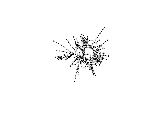
Draw a 494-vertex power network from the SuiteSparse Matrix Collection. The graph is bundled with grip: no download or matrix conversion is needed. Browse all 85 bundled graphs with suitesparse.graphs(); its gallery column identifies the 80 curated comparison graphs. Edges come from the matrix’s nonzero off-diagonal pattern and have unit length; matrix coefficients are not used as distances. Targets are shortest-path hop counts.

library(grip)
g <- suitesparse.graph("494_bus")

fit <- metric.mds(
  edges = g$edges, n = g$n, dim = 3,
  backend = "sgd", seed = 11
)
#> Warning: Selected metric.mds() start terminated with iteration_limit; budget
#> exhaustion does not certify convergence; inspect metadata$starts
coords <- fit$coords
edges <- g$edges
plot.layout(fit$coords, edges = g$edges, projection = "ortho")

Rotate and explore the power network in the interactive gallery (its saved fits have their own stated settings). For an interactive view of this exact fit in R:

ivue::plot3D.plain(fit$coords,
  layers = list(ivue::layer3D.edges(g$edges)))

This is an embedding of network connectivity, not a geographic map of the power system. Inspect fit$metadata$starts: an iteration-limit warning means coordinates were returned without meeting the stopping criterion. A returned embedding does not establish convergence or an optimum.

Choosing a workflow

Weighted graph distances

Task	Starting point
Fit unweighted or weighted graph distances	`metric.mds(..., backend = "sgd")`
Avoid a full pairwise distance matrix	`metric.mds(..., backend = "sgd", approximation = "sparse")`
Assess an embedding	`score.layout()` and the diagnostics relevant to the application
Compare optimization methods	SGD versus `backend = "smacof"`, on the same full-MDS targets and weights
Explore alternative layouts	Classical MDS or multiscale GRIP; see below

Supply positive edge lengths, not connection strengths. Full MDS uses shortest paths computed from these lengths.

weighted.edges <- cbind(1:3, 2:4)
weighted.fit <- metric.mds(
  edges = weighted.edges, n = 4, edge.weights = c(1, 2, 1.5),
  dim = 2, backend = "sgd", seed = 12, diagnostics = FALSE
)
#> Warning: Selected metric.mds() start terminated with iteration_limit; budget
#> exhaustion does not certify convergence; inspect metadata$starts

Sparse MDS for larger graphs

Sparse mode retains graph edges and represents longer-range influences using selected vertices called pivots. Pass graph inputs directly rather than preparing a dense distance matrix first.

large.edges <- edges.mesh(20, 20)
sparse.fit <- metric.mds(
  edges = large.edges, n = 400, dim = 3,
  backend = "sgd", approximation = "sparse", seed = 3,
  sparse.control = list(n.pivots = 32), max.iter = 100
)

This modest example demonstrates the API; it is not a threshold for switching to sparse mode. Choose according to graph size, memory and accuracy needs. More pivots cost more and do not guarantee improvement in every run.

Sparse mode currently requires a connected graph, uses inverse-squared stress weights, and supports SGD only. Its fitted proxy stress is not directly comparable with full-MDS stress. For weighted graphs, a supplied edge longer than an alternative route can also have a different target in sparse and full MDS. See the sparse guide for constraints, diagnostics and measured examples.

Assess the result

Evaluate the aspect of geometry that matters to the application, rather than choosing a drawing by appearance alone.

quality <- score.layout(coords, edges = edges, n = g$n,
                        sample.size.stress = 200, stress.seed = 11,
                        edge.crossings = "never")
quality[, c("sampled.stress", "edge.length.cv")]
#>   sampled.stress edge.length.cv
#> 1      0.1258268      0.3295209

Sampled stress compares drawn separations with graph hop distances after fitting a common scale; zero means exact agreement on the sampled pairs. The edge-length coefficient of variation measures relative variation in drawn edge lengths, useful here because the graph is unweighted. Neither measure certifies recovery of a reference shape, and this assessment stress need not match the optimizer’s weighted objective.

For method comparisons, hold graph inputs, target distances and evaluation pairs fixed where applicable. Report seeds and computational budgets. For sparse MDS, evaluate against independently selected shortest-path targets rather than comparing sparse proxy values across pivot counts.

Do not append edge-KK automatically. It changes the fitting objective; retain an additional refinement only when its diagnostics support the intended use. See Choose a score.

Other layout methods

GRIP presets ("mesh", "carpet", "tree", "torus") configure that algorithm, not metric MDS. For GRIP specifically, metric = "hop" uses hops for hierarchy and neighborhoods; metric = "edge_length" uses supplied positive lengths throughout its weighted shortest-path hierarchy. See the function guide.

Comparing GRIP presets

compare.layouts() can compare GRIP candidates across seeds. The example below compares GRIP presets; it does not compare SGD, sparse MDS and GRIP.

comparison.edges <- edges.mesh(4, 5)
cmp <- compare.layouts(comparison.edges, n = 20, dim = 2,
                       candidates = c("default", "mesh"), seeds = 1:3)
cmp$summary[, c("candidate", "score.composite", "sampled.stress.mean")]

Gallery

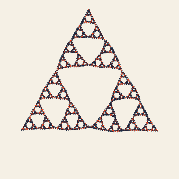
A completed Sierpinski triangle layout. Play the trace on the website to see vertices introduced and refined.

This construction animation illustrates GRIP, an alternative method in the package. The showcase recipes also include carpet traces and saddle rotations. Construction traces show algorithm steps; rotations show saved coordinates. Each example retains its actual fitting provenance.

Documentation

Use vignette(package = "grip") to discover offline guides in an installation built with vignettes. The website includes additional articles and galleries.

Citation

Use citation("grip") for the package citation, and cite the methods used in your analysis. Relevant algorithm references include:

License

Development

The developer map traces graph validation, preparation, engines, results, and displays, and lists source regeneration and full-dependency checks. The recommended embedding workflow is metric.mds() → fit$coords → visualization and independent assessment.