godley

godley is an R package for simulating stock-flow consistent (SFC) macroeconomic models.

By employing godley, users can create fully fledged post-keynesian and MMT models of the economy to:

• analyze the sensitivity of parameter changes,
• impose policy or exogenous shocks,
• visualize diverse dynamic macroeconomic scenarios, and
• study the implications of various macroeconomic structures on key variables.

The package offers the flexibility to support both theoretical frameworks and data-driven scenarios.

It is named in honor of Wynne Godley (1926–2010), a prominent British post-Keynesian economist and a leading figure in SFC modeling.

Installation ⚙️

godley is currently hosted on GitHub github.com/gamrot/godley. To install the development version directly, please use devtools package:

install.packages("devtools")
devtools::install_github("gamrot/godley")

Example 📊

The following demonstrates a basic example of using the package to simulate a baseline scenario in the classic SIM model (Godley & Lavoie, Monetary Economics, 2007).

To define the model structure, start by creating an empty model with the create_model() function.
The resulting model is an S3 object (a list) of the SFC class.

model_sim <- create_model(name = "SFC SIM")

Use the add_variable() function to include variables in the model. This function creates a $variables tibble within the model.

⚠️ Remarks:

• The following characters are not permitted in variable names: §, £, @, #, $, {, }, ;, :, ', \, ~, `, ?, !, %, ^, &, *, (, ), -, +, =, [, ], |, <, ,, >, /.
  
• For best practices, use only letters, numbers, and underscores (_) when naming variables.
  
• Each variable can be initialized with either a single scalar (representing a theoretical starting point) or a full vector of real data.

model_sim <- model_sim |>
 add_variable("C_d", desc = "Consumption demand by households") |> 
 add_variable("C_s", desc = "Consumption supply") |> 
 add_variable("G_s", desc = "Government supply") |> 
 add_variable("H_h", desc = "Cash money held by households") |> 
 add_variable("H_s", desc = "Cash money supplied by the government") |> 
 add_variable("N_d", desc = "Demand for labor") |> 
 add_variable("N_s", desc = "Supply of labor") |> 
 add_variable("T_d", desc = "Taxes, demand") |> 
 add_variable("T_s", desc = "Taxes, supply") |> 
 add_variable("Y", desc = "Income = GDP") |> 
 add_variable("Yd", desc = "Disposable income of households") |> 
 add_variable("alpha1", init = 0.6, desc = "Propensity to consume out of income") |> 
 add_variable("alpha2", init = 0.4, desc = "Propensity to consume out of wealth") |> 
 add_variable("theta", init = 0.2, desc = "Tax rate") |> 
 add_variable("G_d", init = 20, desc = "Government demand") |> 
 add_variable("W", init = 1, desc = "Wage rate")

model_sim$variables

## # A tibble: 16 × 3
##    name   init      desc
##    <chr>  <list>    <chr>
##  1 C_d    0         Consumption demand by households
##  2 C_s    0         Consumption supply
##  3 G_s    0         Government supply
##  4 H_h    0         Cash money held by households
##  5 H_s    0         Cash money supplied by the government
##  6 N_d    0         Demand for labor
##  7 N_s    0         Supply of labor
##  8 T_d    0         Taxes, demand
##  9 T_s    0         Taxes, supply
## 10 Y      0         Income = GDP
## 11 Yd     0         Disposable income of households
## 12 alpha1 0.6       Propensity to consume out of income
## 13 alpha2 0.4       Propensity to consume out of wealth
## 14 theta  0.2       Tax rate
## 15 G_d    20        Government demand
## 16 W      1         Wage rate

Then, specify the system of equations that governs the model. This can be done using the add_equation() function by providing the equations in text form. The model will then include a $equations tibble.

Equations must adhere to the following rules:

1. The following characters are not allowed: §, £, @, #, $, {, }, ;, :, ', \, ~, `.
   
2. Some characters are acceptable but treated as operators (ignored when reading variable names): !, %, ^, &, *, (, ), -, +, =, [, ], |, <, ,, >, /.
   
3. The left-hand side must contain a variable that the equation defines, written in its untransformed form. For example, C_s for consumption. Constructs like C_s*2 or log(C_s) are not allowed on the left-hand side. If an operator or function appears on the left, the entire expression will be treated as the variable name.
4. An equals sign = must separate the left-hand side from the right-hand side.
5. The right-hand side should contain the rest of the equation, written using variable names, standard operators, and functions available in R. For convenience, the package also includes commonly used operations on matrix columns, such as lags and differences:
   • Lags: Add a negative lag order in square brackets to a variable. For example, the first lag of consumption is written as C_s[-1], and the third lag as C_s[-3]. The package supports lags up to the fourth order, which is particularly useful for quarterly data. This syntax mirrors the behavior of the lag() function in R.
   • First differences: The first difference, e.g., C_s - C_s[-1], can be written as d(C_s). This is equivalent to the diff() function in R. Note that this operation is defined only for the first difference; higher-order differences, such as the third difference, must be expressed explicitly, e.g., C_s - C_s[-3].
   • Lagged differences: Combine the above two operations, e.g., d(C_s[-1]).
6. Each variable being defined can appear on the left-hand side of a single equation. It is not allowed to have multiple different equations for the same variable (exact duplicates are flagged with an appropriate message).

model_sim <- model_sim |>
  add_equation("C_s = C_d", desc = "Consumption") |> 
  add_equation("G_s = G_d") |> 
  add_equation("T_s = T_d") |> 
  add_equation("N_s = N_d") |> 
  add_equation("Yd = W * N_s - T_s") |> 
  add_equation("T_d = theta * W * N_s") |> 
  add_equation("C_d = alpha1 * Yd + alpha2 * H_h[-1]") |> 
  add_equation("H_s = G_d - T_d + H_s[-1]") |> 
  add_equation("H_h = Yd - C_d + H_h[-1]") |> 
  add_equation("Y = C_s + G_s") |> 
  add_equation("N_d = Y/W") |> 
  add_equation("H_s = H_h", desc = "Money equilibrium", hidden = TRUE)

model_sim$equations

## # A tibble: 12 × 3
##    equation                             hidden desc               
##    <chr>                                <lgl>  <chr>              
##  1 C_s = C_d                            FALSE  "Consumption"      
##  2 G_s = G_d                            FALSE  ""                 
##  3 T_s = T_d                            FALSE  ""                 
##  4 N_s = N_d                            FALSE  ""                 
##  5 Yd = W * N_s - T_s                   FALSE  ""                 
##  6 T_d = theta * W * N_s                FALSE  ""                 
##  7 C_d = alpha1 * Yd + alpha2 * H_h[-1] FALSE  ""                 
##  8 H_s = G_d - T_d + H_s[-1]            FALSE  ""                 
##  9 H_h = Yd - C_d + H_h[-1]             FALSE  ""                 
## 10 Y = C_s + G_s                        FALSE  ""                 
## 11 N_d = Y/W                            FALSE  ""                 
## 12 H_s = H_h                            TRUE   "Money equilibrium"

With all variables and equations defined, the model is ready to be solved over a given time horizon. This can be done using the simulate_scenario() function. The function starts by validating the user-defined model through the prepare() function, which is also accessible in the package’s exported environment.

The function allows choosing a simulation method (Newton or Gauss), selecting the number of periods and a starting date. Specifying an initial period is optional; if omitted, periods will simply be numbered consecutively with natural numbers.

By default, equations are solved using the Gauss method. Independent equations for a specific period are resolved in a single iteration. Interdependent equations are grouped into loops and solved iteratively. For the first period, the method uses the provided initial values (init). In subsequent iterations, it relies on the results of the previous iteration for all variables. The process continues until the solution converges within the specified tolerance (tol) or the maximum number of iterations (max_iter) is reached. If any period produces a value of Inf, NaN, or NA, the process is stopped, and an error message is displayed.

Before solving equations, their order is determined to:

1. Solve endogenous variables first, allowing them to be used as exogenous variables later.
   
2. Group interdependent equations into loops, ensuring proper substitution of exogenous variables.

The Newton method works similarly but uses the Newton-Raphson algorithm to solve interdependent equations. This algorithm is implemented via the rootSolve::multiroot() function.

During the model-building phase, setting the info = TRUE argument can be helpful. This returns the result of the prepare() function, providing details on the classification of all variables (endogenous/exogenous) and other summary information about the input data.

Simulation results are saved in a $result tibble linked to the scenario being simulated (e.g., the baseline scenario is stored as $baseline).

model_sim <- model_sim |>
  simulate_scenario(
    periods = 100, start_date = "2015-01-01",
    method = "Gauss", max_iter = 350, tol = 1e-05
  )

model_sim$baseline$result

## # A tibble: 100 × 17
##    time         C_s   G_s   T_s   N_s    Yd   T_d   C_d   H_s   H_h     Y   N_d
##    <date>     <dbl> <dbl> <dbl> <dbl> <dbl> <dbl> <dbl> <dbl> <dbl> <dbl> <dbl>
##  1 2015-01-01   0       0  0      0     0    0      0     0     0     0     0  
##  2 2015-04-01  18.5    20  7.69  38.5  30.8  7.69  18.5  12.3  12.3  38.5  38.5
##  3 2015-07-01  27.9    20  9.59  47.9  38.3  9.59  27.9  22.7  22.7  47.9  47.9
##  4 2015-10-01  35.9    20 11.2   55.9  44.8 11.2   35.9  31.5  31.5  55.9  55.9
##  5 2016-01-01  42.7    20 12.5   62.7  50.2 12.5   42.7  39.0  39.0  62.7  62.7
##  6 2016-04-01  48.5    20 13.7   68.5  54.8 13.7   48.5  45.3  45.3  68.5  68.5
##  7 2016-07-01  53.3    20 14.7   73.3  58.6 14.7   53.3  50.6  50.6  73.3  73.3
##  8 2016-10-01  57.4    20 15.5   77.4  61.9 15.5   57.4  55.2  55.2  77.4  77.4
##  9 2017-01-01  60.9    20 16.2   80.9  64.7 16.2   60.9  59.0  59.0  80.9  80.9
## 10 2017-04-01  63.8    20 16.8   83.8  67.1 16.8   63.8  62.2  62.2  83.8  83.8
## # … with 90 more rows, and 5 more variables: alpha1 <dbl>, alpha2 <dbl>,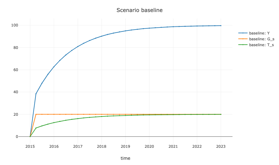
## #   theta <dbl>, G_d <dbl>, W <dbl>

Visualizations 🎨

The godley package provides customized visualization capabilities to enhance the analysis of simulation outcomes.

Users can leverage the plot_simulation() function to create plots, by specifying the time range with from and to, along with a list of expressions. These expressions can include variable names or calculations derived from them, such as G_s/Y. In the example below, the plot displays the expressions for Income, Government Spending, and Taxes.

plot_simulation(
  model_sim, scenario = "baseline",
  from = "2015-01-01", to = "2023-01-01",
  expressions = c("Y", "G_s", "T_s")
)

Beyond plotting variables over time, the plot_cycles() function provides a way to visualize the model’s structure and uncover loops (feedback mechanisms and endogeneity) within the interdependencies between variables, offering an intuitive approach for interpreting and communicating the results of macroeconomic simulations.

plot_cycles(model_sim)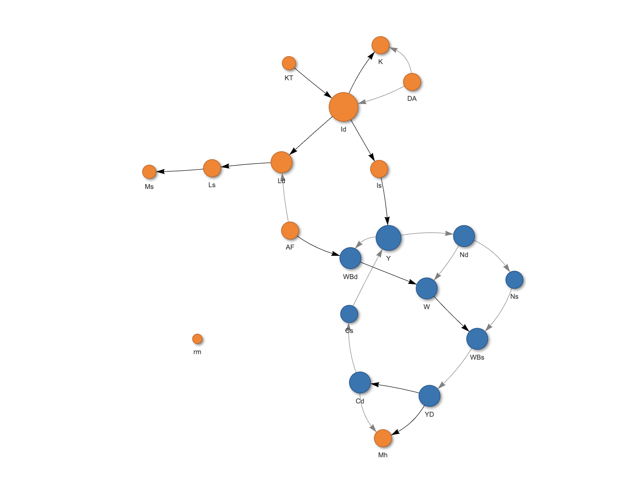

Templates 📝

To streamline model creation, godley comes with predefined templates. Rather than starting with an empty model and manually adding equations each time, users can reuse a previously created model or choose from the classic SFC models (Godley & Lavoie, 2007) included in the package. These templates are available through the template argument in the create_model() function. The available templates include SIM, SIMEX, PC, PCEX, LP, REG, OPEN, BMW, BMWK, DIS, and DISINF, covering all models presented in Godley & Lavoie (2007).

Shocks ⚡

The package allows users to introduce and simulate shocks within the model.

An alternative shock scenario is defined by:

1. Shock parameters (which variable is affected, when it occurs, and what value it takes),
   
2. Simulation (how many future periods the new scenario should cover).

To create a shock, begin by initializing an empty S3 object (list) of the SFC_shock class using the create_shock() function. Next, add the shock parameters for selected variables (variable) using the add_shock() function. Shock values can be defined explicitly (value), as a relative rate (rate), or as an absolute increment (absolute).

For example, a 20% increase in government spending can be simulated by first creating a shock object using create_shock() and then applying it with add_shock() for the period between Q1 2017 and Q4 2020.

sim_shock <- create_shock() |>
  add_shock(
    variable = "G_d", rate = 0.2,
    start = "2017-01-01", end = "2020-10-01",
    desc = "permanent increase in government expenditures"
  )

Once the shock has been defined, it can be incorporated into a new scenario using add_scenario(). The baseline scenario and corresponding time periods must first be specified. After establishing the shock scenario, the simulate_scenario() function can be executed again to generate the updated results.

model_sim <- model_sim |>
  add_scenario(
    name = "expansion", origin = "baseline",
    origin_start = "2015-01-01", origin_end = "2023-10-01",
    shock = sim_shock
  ) |>
  simulate_scenario(periods = 100)

model_sim$expansion$result

## # A tibble: 100 × 17
##    time         C_s   G_s   T_s   N_s    Yd   T_d   C_d   H_s   H_h     Y   N_d
##    <date>     <dbl> <dbl> <dbl> <dbl> <dbl> <dbl> <dbl> <dbl> <dbl> <dbl> <dbl>
##  1 2015-01-01   0       0  0      0     0    0      0     0     0     0     0  
##  2 2015-04-01  18.5    20  7.69  38.5  30.8  7.69  18.5  12.3  12.3  38.5  38.5
##  3 2015-07-01  27.9    20  9.59  47.9  38.3  9.59  27.9  22.7  22.7  47.9  47.9
##  4 2015-10-01  35.9    20 11.2   55.9  44.8 11.2   35.9  31.5  31.5  55.9  55.9
##  5 2016-01-01  42.7    20 12.5   62.7  50.2 12.5   42.7  39.0  39.0  62.7  62.7
##  6 2016-04-01  48.5    20 13.7   68.5  54.8 13.7   48.5  45.3  45.3  68.5  68.5
##  7 2016-07-01  53.3    20 14.7   73.3  58.6 14.7   53.3  50.6  50.6  73.3  73.3
##  8 2016-10-01  57.4    20 15.5   77.4  61.9 15.5   57.4  55.2  55.2  77.4  77.4
##  9 2017-01-01  64.6    24 17.7   88.6  70.9 17.7   64.6  61.4  61.4  88.6  88.6
## 10 2017-04-01  69.4    24 18.7   93.4  74.7 18.7   69.4  66.8  66.8  93.4  93.4
## # … with 90 more rows, and 5 more variables: alpha1 <dbl>, alpha2 <dbl>,
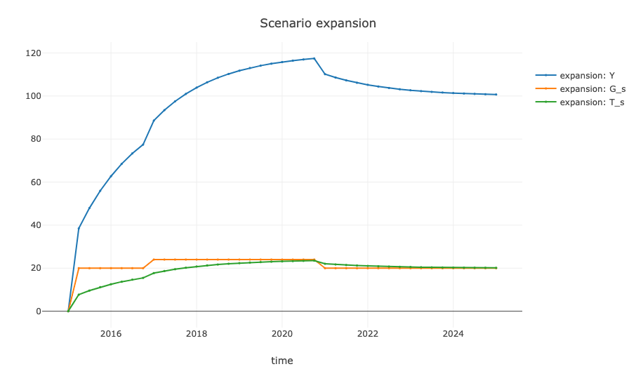
## #   theta <dbl>, G_d <dbl>, W <dbl>

The results indicate that increased government expenditures have a positive effect on income, but a less favorable short-term impact on the government balance. This outcome can be visualized as follows:

plot_simulation(
  model_sim, scenario = "expansion",
  to = "2025-01-01", expressions = c("Y", "G_s", "T_s")
)

Sensitivity 🧙

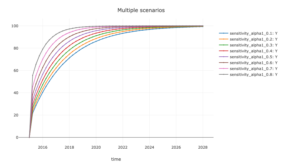
The godley package allows for the assessment of simulation result sensitivity to specific parameter values. For example, the effect of small adjustments to alpha1 on short-term dynamics can be analyzed by first creating a new model object with create_sensitivity() and specifying the upper and lower bounds for the parameter of interest.

The create_sensitivity() function generates a new SFC object based on an existing model and automatically adds multiple scenarios. These scenarios differ only in the value of the selected parameter (variable), which is varied across a specified range defined by lower, upper, and step.

Once the sensitivity scenarios are generated, the simulations can be executed:

model_sens <- model_sim |>
  create_sensitivity(
    variable = "alpha1", lower = 0.1, upper = 0.8, step = 0.1
  ) |>
  simulate_scenario(periods = 100, start_date = "2015-01-01")

The results can be displayed in a plot. To visualize multiple scenarios that share the same scenario substring in their names, set the take_all = TRUE argument.

plot_simulation(
  model_sens, scenario = "sensitivity", take_all = TRUE,
  to = "2028-01-01", expressions = c("Y")
)

Additional examples ⭐

More examples and detailed information about godley functions and model setups are available at the package website.

Key Functions 🔧

• create_model(): Create an SFC model.
• add_variable(): Add variables to the model.
• add_equation(): Add equations to the model.
• simulate_scenario(): Simulate one or more scenarios.
• plot_simulation(): Plot simulation results.
• plot_cycles(): Visualize model structure and feedback loops.
• create_shock(): Create a shock object.
• add_shock(): Add shock parameters.
• add_scenario(): Add a new scenario to an existing model.
• create_sensitivity(): Generate sensitivity scenarios for selected parameters.

Similar work 👪

The following packages also provide approaches to stock-flow consistent modeling:

• sfcr: An alternative framework for SFC modeling.
• bimets: Offers time series and econometric tools for empirical models.
• pysolve3: A Python-based solver for SFC models.

Getting help 🐛

If any issues arise or bugs are encountered, please file a report with a minimal reproducible example at https://github.com/gamrot/godley/issues.