 expertsurv
expertsurv
expertsurv
The goal of expertsurv is to incorporate expert opinion
into an analysis of time to event data. expertsurv uses
many of the core functions of the survHE package (Baio
2020) and also the flexsurv package (Jackson 2016).
Technical details of the implementation are detailed in (Cooney and
White 2023) and will not be repeated here.
The key function is fit.models.expert and operates
almost identically to the fit.models function of
survHE.
You can install the released version of expertsurv from CRAN with:
install("expertsurv")If we have elicited expert opinion of the survival probability at certain timepoint(s) and assigned distributions to these beliefs, we encode that information as follows:
#A param_expert object; which is a list of
#length equal to the number of timepoints
param_expert_example1 <- list()

#If we have 1 timepoint and 2 experts
#dist is the names of the distributions
#wi is the weight assigned to each expert (usually 1)
#param1, param2, param3 are the parameters of the distribution
#e.g. for norm, param1 = mean, param2 = sd
#param3 is only used for the t-distribution and is the degress of freedom.
#We allow the following distributions:
#c("normal","t","gamma","lognormal","beta")


param_expert_example1[[1]] <- data.frame(dist = c("norm","t"),
                                         wi = c(0.5,0.5), # Ensure Weights sum to 1
                                         param1 = c(0.1,0.12),
                                         param2 = c(0.005,0.005),
                                         param3 = c(NA,3))
param_expert_example1
#> [[1]]
#>   dist  wi param1 param2 param3
#> 1 norm 0.5   0.10  0.005     NA
#> 2    t 0.5   0.12  0.005      3

#Naturally we will specify the timepoint for which these probabilities where elicited

timepoint_expert <- 14


#In case we wanted a second timepoint -- Just for illustration

# param_expert_example1[[2]] <- data.frame(dist = c("norm","norm"),
#                                          wi = c(1,1),
#                                          param1 = c(0.05,0.045),
#                                          param2 = c(0.005,0.005),
#                                          param3 = c(NA,NA))
#
# timepoint_expert <- c(timepoint_expert,18)
If we wanted opinions at multiple timepoints we just include append
another list (i.e. param_expert_example1[[2]] with the relevant
parameters) and specify timepoint_expert as a vector of
length 2 with the second element being the second timepoint.
For details on assigning distributions to elicited probabilities and
quantiles see the SHELF package (Oakley 2021) and for an
overview on methodological approaches to eliciting expert opinion see
(O’Hagan 2019). We can see both the individual and pooled distributions
using the following code (note that we could have used the output of the
fitdist function from SHELF if we actually
elicited quantiles from an expert):
plot_opinion1 <- plot_expert_opinion(param_expert_example1[[1]],
                    weights = param_expert_example1[[1]]$wi)
ggsave("Vignette_Example 1 - Expert Opinion.png")
For the log pool we have a uni-modal distribution (in contrast to the bi-modal linear pool) which has a \(95\%\) credible interval between \(9.0−11.9\%\) calculated with the function below:
cred_int_val <- cred_int(plot_opinion1,val = "log pool", interval = c(0.025, 0.975))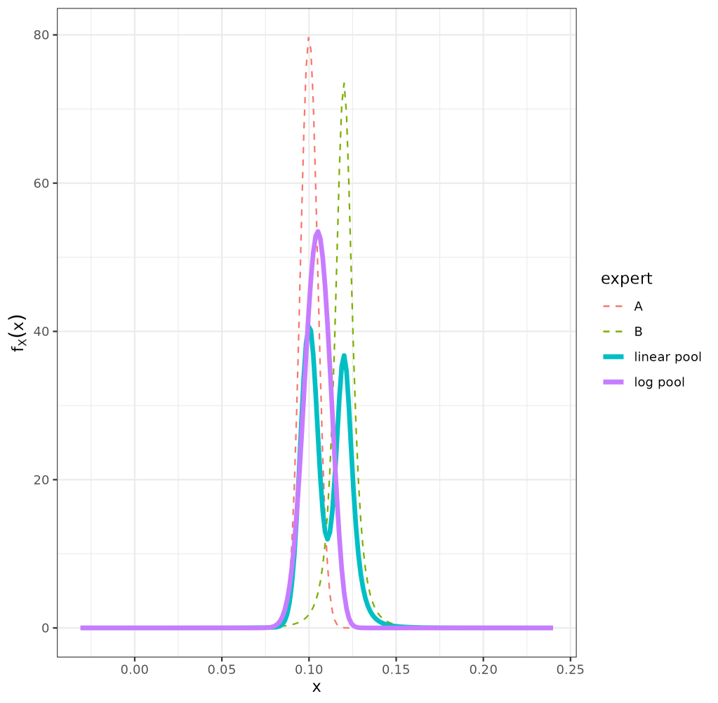
Expert prior distributions
We load and fit the data as follows (in this example considering just
the Weibull and Gompertz models), with
pool_type = "log pool" specifying that we want to use the
logarithmic pooling (rather than default “linear pool”). We do this as
we wish to compare the results to the penalized maximum likelihood
estimates in the next section. The stan models are not compiled at
installation, in fact, they are accessed as saved objects from the
inst folder. Therefore, it is much quicker to include the
extra argument compile_mods = compiled_models_saved than
requiring stan to recompile the model at each evaluation.
Because of CRAN’s package size limitations (< 5Mb) it is not possible to include this in the data folder, therefore, this should be compiled when the package is first installed.
# After installation
 compiled_models_saved <- expertsurv:::compile_stan()
 path_all <- system.file("data",package = "expertsurv")
 save(compiled_models_saved, file = paste0(path_all,"/compiled_stan.RData"), compress = "xz")

# At start of session
load(paste0(paste0(path_all,"/compiled_stan.RData")))


data2 <- data %>% rename(status = censored) %>% mutate(time2 = ifelse(time > 10, 10, time),
                                                              status2 = ifelse(time> 10, 0, status))

#Set the opinion type to "survival"

example1  <- fit.models.expert(formula=Surv(time2,status2)~1,data=data2,
                               distr=c("wph", "gomp"),
                               method="bayes",
                               iter = 5000,
                               pool_type = "log pool",
                               opinion_type = "survival",
                               times_expert = timepoint_expert,
                               param_expert = param_expert_example1,
                               compile_mods = compiled_models_saved)
Both visual fit and model fit statistics highlight that the Weibull model is a poor fit to both the expert opinion and data (black line referring to the \(95\%\) confidence region for the experts prior belief).
The below code provides the goodness of fit (in this case DIC,
however, I prefer WAIC or PML). Also presented is the survival plots, at
the posterior mean values. If opinion was included on survival outcomes
it can be helpful to visualize the density of the expert opinion by
plot_opinion = TRUE. Statistical uncertainty can also be
plotted using the plot_ci = TRUE argument and by specifying
nsim equal to however many simulations you desire (for
Bayesian models this must be less than the total number of simulations
from the posterior). By default the confidence/credible intervals are
plotted as dashed lines, however, if an area/ribbon plot is preferred
then set ci_plot_ribbon = TRUE.
Even if statistical uncertainty is not required in the plots, I
recommend nsim is set to a reasonable number. If
nsim = 1 as by default, the maximum likelihood estimates or
the posterior mean of the parameters will be used to plot the results.
In most cases this should suffice (particularly for maximum likelihood),
however, the expected survival estimated by the full sampling
distribution may be different to the estimate at it’s expectation/max
likelihood estimate. This more likely in the Bayesian analysis if the
posterior is non-normal. In the below plot the results for both
approaches are similar and therefore, we omit these arguments.
model.fit.plot(example1, type = "dic") #Also "waic" or "pml"
plot(example1, add.km = T, t = 0:30,plot_opinion  = TRUE)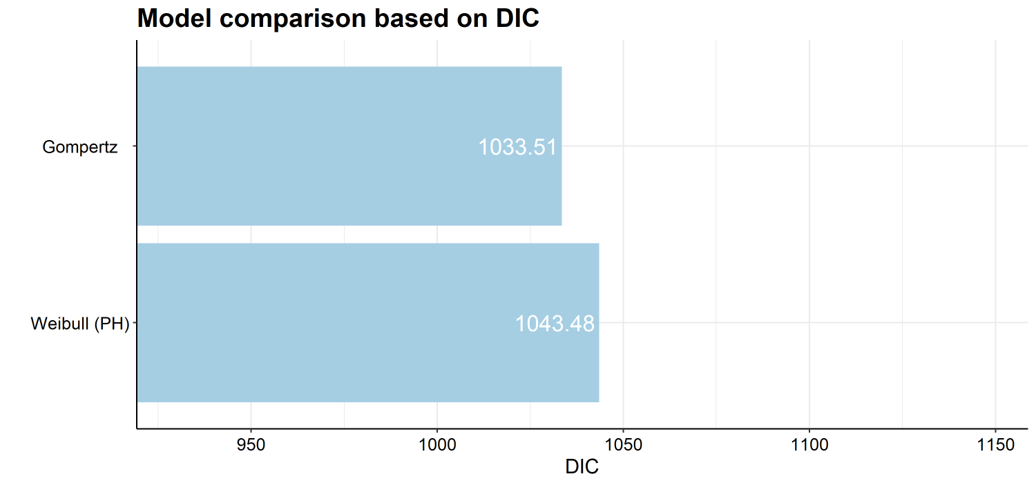
Model Comparison
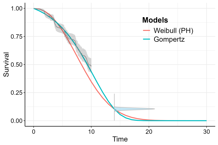
Survival function with Expert prior
We can also fit the model by Penalized Maximum Likelihood approaches
based on code taken from the flexsurv package (Jackson
2016). All that is required that the method="bayes" is
changed to method="mle" with the iter argument
now redundant. One argument that maybe of interest is the
method_mle which is the optimization procedure that
flexsurv uses. In case the optimization fails, we can
sometimes obtain convergence with the Nelder-Mead
algorithm. If the procedure is still failing, it may relate to the
expert opinion being too informative.
It should be noted that the results will be similar to the Bayesian approach when the expert opinion is unimodal and relatively more informative, therefore we use the logarithmic pool which is unimodal.
We find that the AIC values also favour the Gompertz model by a large factor (not shown) and are very similar to the DIC presented for the Bayesian model.
In this situation we place an opinion on the comparator arm. In this
example id_St is used to specify the row number in the data
frame of the comparator arm, indicating that the covariate pattern for
this row represents the group for which the expert opinion is
provided.
param_expert_example2[[1]] <- data.frame(dist = c("norm"),
wi = c(1),
param1 = c(0.1),
param2 = c(0.005),
param3 = c(NA))
#Check the coding of the arm variable
#Comparator is 0, which is our id_St
unique(data$arm)
[1] 0 1
#We want our opinion to refer to the treatment called "0"
example2 <- fit.models.expert(formula=Surv(time2,status2)~as.factor(arm),
data=data2,
distr=c("wei"),
method="bayes",
iter = 5000,
opinion_type = "survival",
id_St = min(which(data2$arm ==0)),
times_expert = timepoint_expert,
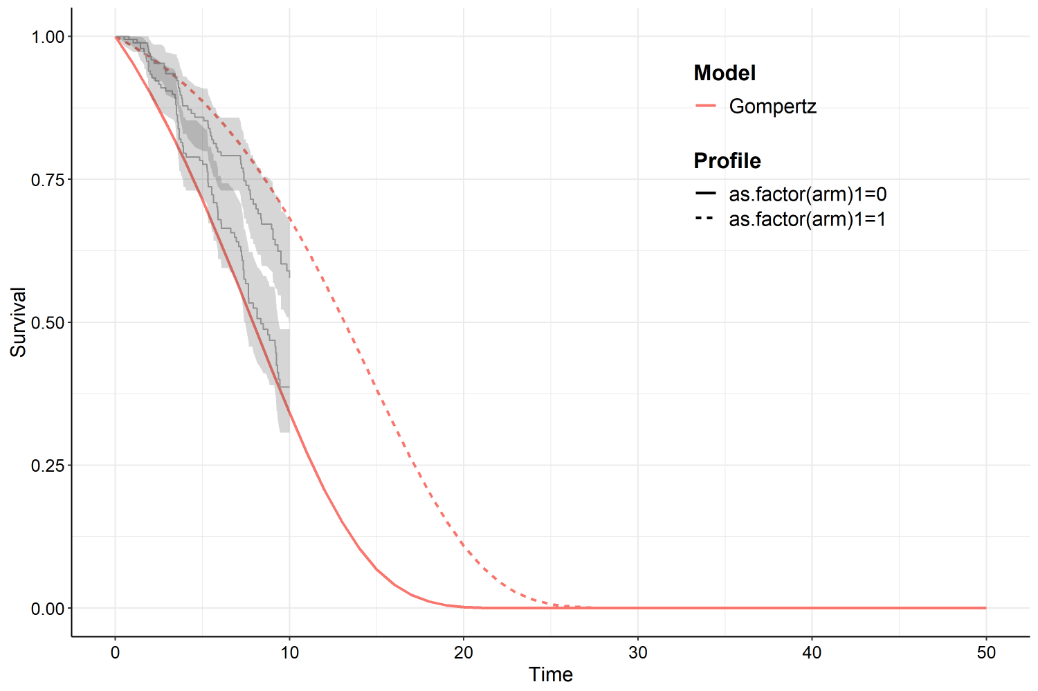
param_expert = param_expert_example2)We can remove the impact of expert opinion omitting the arguments
relating to opinion_type,id_St,times_expert,param_expert,
\(\dots\) with the function.
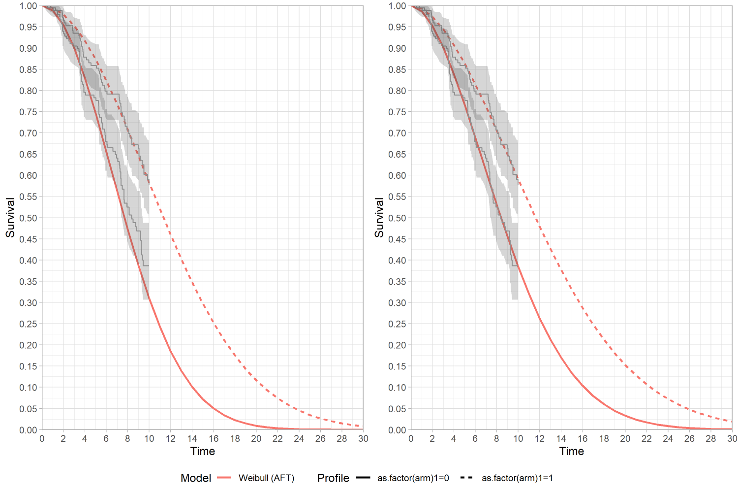
Survival function with Expert prior (left) and Vague prior (right)
The survival function for “arm 1” has been shifted downwards slightly, however the covariate for the accelerated time factor has markedly increased to counteract the lower survival probability for the reference (arm 0).
This example illustrates an opinion on the survival difference. For illustration we use the Gompertz, noting that a negative shape parameter will lead to a proportion of subjects living forever. Clearly the mean is not defined in these cases so the code automatically constrains the shape to be positive. It should also be noted that there are many potential combinations of survival curves which could produce a difference in the expected survival of 5 months. If this approach is considered, the number of iterations should be quite large to ensure convergence.
param_expert3 <- list()

#Prior belief of 5 "months" difference in expected survival
param_expert3[[1]] <- data.frame(dist = "norm", wi = 1, param1 = 5, param2 = 0.2, param3 = NA)


survHE.data.model  <- fit.models.expert(formula=Surv(time2,status2)~as.factor(arm),data=data2,
                                                     distr=c("gom"),
                                                     method="bayes",
                                                     iter = 5000,
                                                     opinion_type = "mean",
                                                     id_trt = min(which(data2$arm ==1)), # Survival difference is  Mean_surv[id_trt]- Mean_surv[id_comp]
                                                     id_comp = min(which(data2$arm ==0)),
                                                     param_expert = param_expert3)
Survival difference
As stated in the introduction this package relies on many of the core
functions of the survHE, flexsurv packages (Baio 2020) and
(Jackson 2016). Because future versions of survHE and
flexsurv may introduce conflicts with the current
implementation, we have directly ported the key functions from these
packages into the package so that expertsurv no longer
imports survHE,flexsurv (of course all credit for those
functions goes to Jackson (2016)).
If you run in issues, bugs or just features which you feel would be useful, please let me know (phcooney@tcd.ie) and I will investigate and update as required.
As this is a Bayesian analysis convergence diagnostics should be performed. Poor convergence can be observed for many reasons, however, because of our use of expert opinion it may be a symptom of conflict between the observed data and the expert’s opinion.
Default priors should work in most situations, but still need to be considered. At a minimum the Bayesian results without expert opinion should be compared against the maximum likelihood estimates. If considerable differences are present the prior distributions should be investigated.
Because the analysis is done in JAGS and Stan we can leverage the
ggmcmc package (Fernández-i-Marín 2016):
library(ggmcmc)
#For Stan Models # Log-Normal, RP, Exponential, Weibull
ggmcmc(ggs(rstan::As.mcmc.list(example1$models$`Exponential`)), file = "Exponential.pdf")

#For JAGS Models # Gamma, Gompertz, Generalized Gamma
ggmcmc(ggs(as.mcmc(example1$models$`Gamma`)), file = "Gamma.pdf")Please note that this functionality is still in an experimental stage
Because expertsurv uses flexsurv functions
internally the models fit by penalized maximum likelihood
method = "mle" inherit the flexsurvreg class.
This means that we can leverage advanced approaches such as the
inclusion of general population mortality. This is discussed in more
detail in the package documentation of the flexsurv package
and more specifically the standsurv vignette (Sweeting
2023), however, the key point to note is that the parameter estimates
obtained from the survival models are for the relative survival
model and therefore are not representative of the all-cause survival
(which typically considers the disease specific and general population
mortality hazards).
After making the modifications to the bc dataset as in
the standsurv vignette, we assume a the expert believes
that the expected survival for the “Good” group is \(40\%\) with a standard deviation of \(5\%\) and can be characterized by a Normal
distribution at 20 years.
We fit a Gompertz distribution and note the survival below.
timepoint_expert <- 20

example1  <- fit.models.expert(formula=Surv(recyrs,censrec)~as.factor(group2),data=bc,
                               distr=c("gomp"),
                               method="mle",
                               opinion_type = "survival",
                               times_expert = timepoint_expert,
                               param_expert = param_expert_example1,
                               id_St = min(which(bc$group2 =="Good")))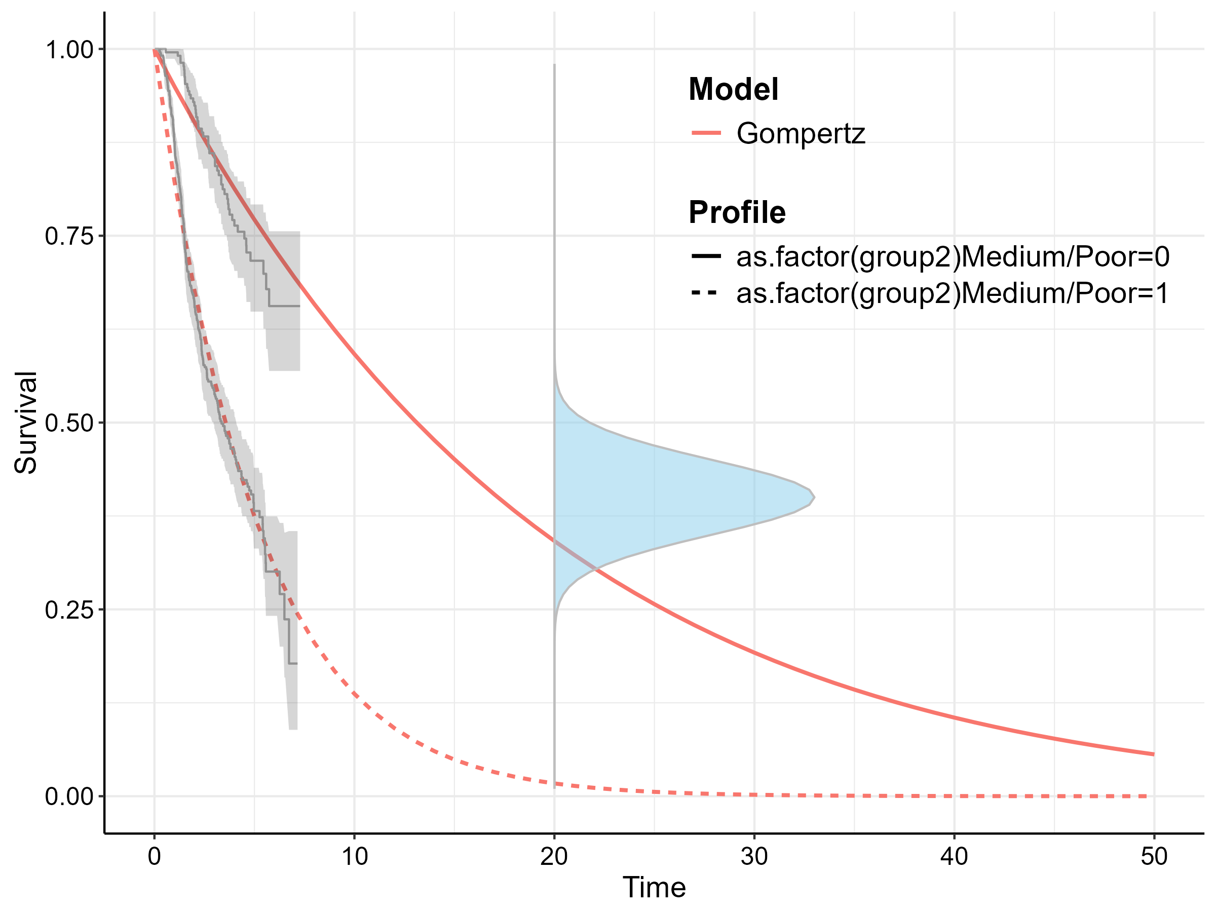
Survival Estimates without General Population Mortality
We have not, however, considered the impact of general population
mortality, and in this example the expected survival of the general
population is approximately \(50\%\).
Therefore, the expert’s belief that the expected survival of the “Good”
group is \(40\%\) implies that the
hazard of the this group approaches that of the general population. To
include this, we first need to extract the parameters of the expert
opinion that were used in the previous model (I don’t currently have a
function to do this without running the fit.models.expert
first).
The survival of the general population at the elicited timepoint is
added to the expert_opinion_flex list and supplied to the
exposed expertsurv:::flexsurvreg function (this is the
flexsurvreg function which is only available internally to
the expertsurv package and so does not conflict with
flexsurv::flexsurvreg). Furthermore, we no longer assume
proportional hazards so that we can illustrate the hazards of the “Good”
group.
expert_opinion_flex <- example1$misc$flex_expert_opinion[[1]]
expert_opinion_flex$bhazard_par <- c(0.5)

model.gomp.sep.rs <- expertsurv:::flexsurvreg(Surv(recyrs, censrec)~as.factor(group2),
                                     data=bc, dist="gompertz",
                                     anc = list(shape = ~ as.factor(group2)),
                                     bhazard=exprate,expert_opinion = expert_opinion_flex)
Using the standsurv functions (as documented by
(Sweeting 2023)) we can generate the all-cause hazards and survival.
While the all cause survival is broadly similar to the predicted
survival for the “Good” group without general population mortality
adjustment at the timepoint of 20 years, the adjustment ensures that the
“Good” group survival does not exceed the general population mortality
which would be the case at a timepoint of 30 years.
Although theoretically possible, the general population mortality adjustment has not been implemented for the situation when expert opinion is provided for differences in mean survival.
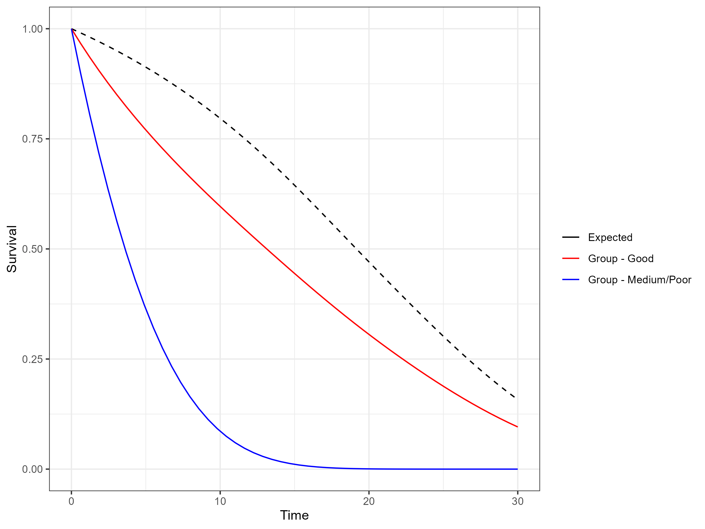
All-cause Survival Estimates including General Population Mortality
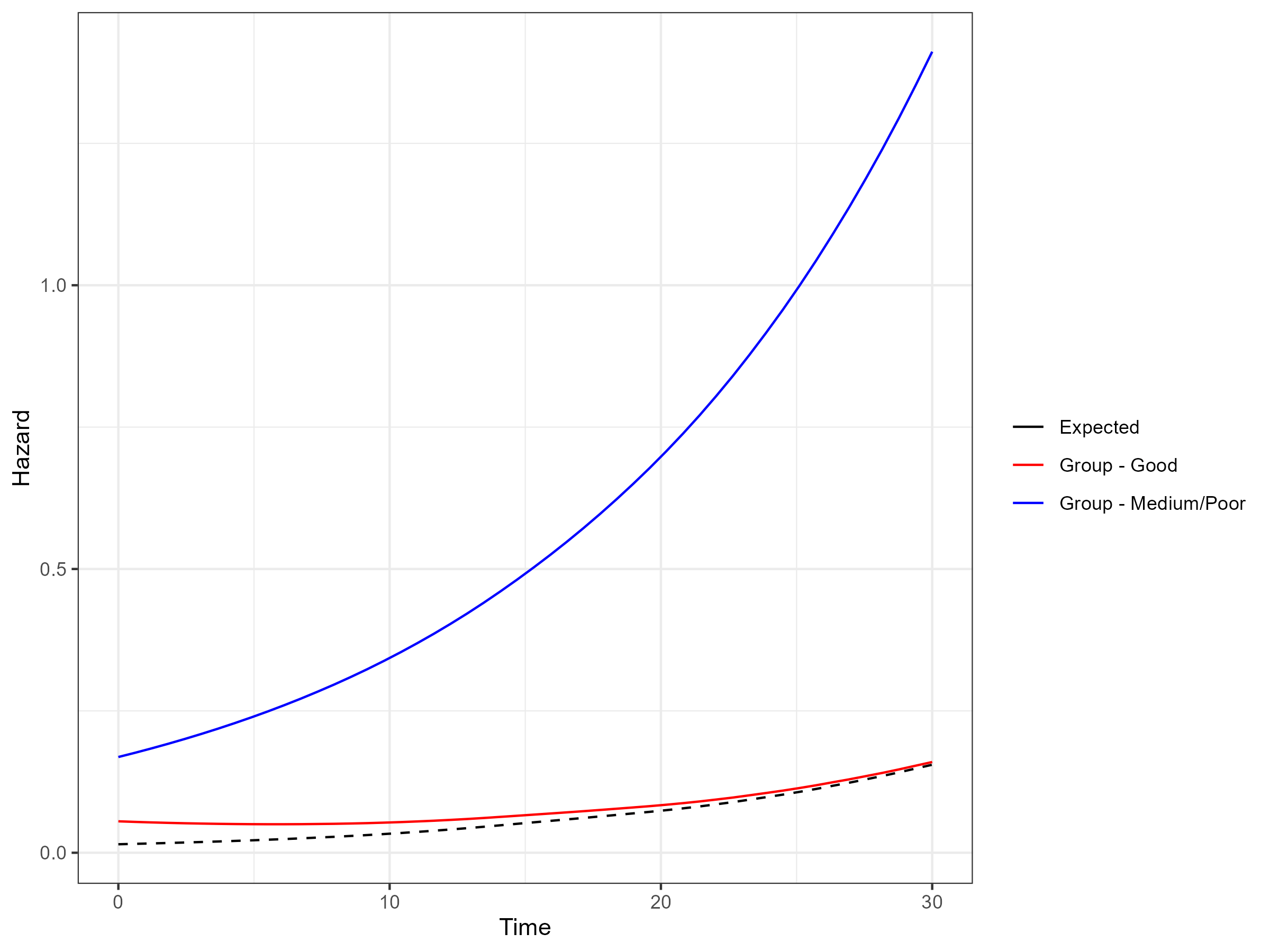
All-cause Hazard Functions including General Population Mortality
In most cases, the models are estimated successfully. However, there
are instances where the choice of initial values is crucial. This is
especially significant for the Gompertz model when using Bayesian
methods. The Gompertz model is fit using the zero’s trick
(since it is not available as a probability distribution in JAGS). To
mitigate these issues, expertsurv fits the Gompertz model
using penalized maximum likelihood and then uses these penalized maximum
likelihood estimates as initial values for the Bayesian approach.
If this approach also fails, user-defined initial values can be provided as shown below.
#alpha is the same as the shape parameter in the flexsurv Gompertz model
#beta is the same as the log(rate) parameter flexsurv Gompertz model.
#beta can also include the log(HR) for any covariates
alpha <- 1
beta <- 1

#beta needs to be a vector of length equal to H
#H is 2 whether or not one covariate has been included, however,
#if more than one covariate is included it is the number of covariates +1.
#It can also be accessed from a successfully fit Bayesian model.
#example1_bayes[["misc"]][["data.stan"]][[1]]["H"]

H <- 2
if(data.jags$H > length(beta)){
  beta <- c(beta, rep(0,H-length(beta)))
}

modelinits <- function(){
  list(alpha1 = alpha1,alpha2 = alpha2, beta = beta)
}
#Finally create a function supplying these initial values and then supply
#them as a list with the name of the sublist being the model (i.e. gom)

example1_bayes  <- fit.models.expert(formula=Surv(time2,status2)~1,data=data2,
                                     distr=c("wei", "gom", "lno","llo","gam","wph","exp", "rps"),
                                     method="bayes",
                                     opinion_type = "survival",
                                     times_expert = timepoint_expert,
                                     param_expert = param_expert_example1,
                                     iter = 10000,
                                     k = 1,
                                     knots = c(-1,0,0.5),
                                     a0 = rep(0.0001, 3),
                                     init = list(gom = modelinits),
                                     compile_mods = compiled_models_saved,
                                     expert_only = F)
Supplying initial values for models fit by penalized maximum likelihood is straightforward. By default, initial values for the model with expert opinion are taken from a model fit without data (this happens internally). However, there may be situations where the user wants to supply their own initial values.
For example, if you wish to include expert opinion that is both strong (i.e., the distribution represents the belief with low variance) and significantly different from the survival generated based on data alone, setting the initial values to be equal to the maximum likelihood estimates may result in optimization failure.
In such cases, it may make sense to first fit the model to the data
with an expert opinion having the same expected value (i.e., mean of the
distribution representing their belief) but a larger variance. The
values obtained from this model could then be used as initial values for
the model with the stronger expert opinion. Note that setting initial
values (inits) is not implemented for the spline-based
models.
require("dplyr")
#Expert Opinion as a normal distribution centered on 0.1 with sd 0.005
param_expert_example1 <- list()
param_expert_example1[[1]] <- data.frame(dist = c("norm"),
                                         wi = c(1), # Ensure Weights sum to 1
                                         param1 = c(0.1),
                                         param2 = c(0.01),
                                        param3 = c(NA))
timepoint_expert <- 14 # Expert opinion at t = 14

data2 <- data %>% rename(status = censored) %>% mutate(time2 = ifelse(time > 10, 10, time),
status2 = ifelse(time> 10, 0, status))

#Set the expert opinion to be less strong... i.e. greater variance
param_expert_example1_vague <- param_expert_example1
param_expert_example1_vague[[1]][,4] <- 0.1

example1_vague  <- fit.models.expert(formula=Surv(time2,status2)~1,data=data2,
                              distr=c("wei", "gom"),
                              method="mle",
                              opinion_type = "survival",
                              times_expert = timepoint_expert,
                              param_expert = param_expert_example1_vague)


example1  <- fit.models.expert(formula=Surv(time2,status2)~1,data=data2,
                               distr=c("gom","wei"),
                               method="mle",
                               opinion_type = "survival",
                               times_expert = timepoint_expert,
                               param_expert = param_expert_example1,
                               init = list(gomp = example1_vague$models$Gompertz$res[,1],
                                           wei = example1_vague$models$`Weibull (AFT)`$res[,1]))
The approach of (Cooney and White 2023) integrates the expert opinion by considering inclusion of the expert opinion in terms of a loss function, however, the information could also be formulated as a valid prior distribution.
Consider an expert who has a belief that expected survival of a population at 10 years (\(t^*\)) is normally distributed with a mean of 0.1 (\(\mu_{expert}\)) and standard deviation of 0.05 \(\sigma_{expert}\). To implement this as a prior density we treat the parameters of the expert’s opinion as hyperpriors.
The density of this prior is specific to the survival model that we are estimating and we will first consider the exponential model with parameter \(\theta\) and survival at the expert’s elicited time of \(S(t^*) = \exp\{{-\theta t^*\}}\). Setting the density of the prior to be \(\pi(\theta|\mu_{expert},\sigma_{expert}) \propto \exp\left\{ -\frac{1}{2}\left(\frac{\exp(-\theta t^*) - \mu_i}{\sigma_i}\right)^2 \right\}\). This prior provides the the same density as including the information as a loss function and setting the prior on \(\theta\) to uniform over the support of \(\theta\) (i.e. \([0,\infty)\)).
It is important to recognize that a uniform density on a parameter will not imply a uniform density on a transformation of that parameter. For the one parameter model this is straightforward to calculate via the change of variables technique. Defining \(g(\theta)\) as the survival function of the exponential model, the inverse function of \(g(\theta)\) is \(g^{-1}(\theta) = \frac{-\log(S(t))}{t^*}\), we see that the density of \(S(t^*)\) implied by a uniform prior is \(|g^{-1}(\theta)|\) which is clearly non-uniform (with \(|x|\) denoting the absolute value of \(x\)). For the model with the expert opinion as a normal distribution we can use the change-of-variables technique but in the opposite direction, i.e. given a normal density of the survival what is associated density for the parameter (\(\theta\)). We see that the density of this function is \(\exp\left\{ -\frac{1}{2}\left(\frac{\exp(-\theta t^*) - \mu_i}{\sigma_i}\right)^2 \right\}|g'(\theta)|\) where \(g'(\theta)\) is the derivative of the survival function with respect to \(\theta\).
In the case of a multiparameter model (e.g. Weibull), with parameter vector \(\mathbf{\theta_m}\) of dimension \(m\), \(g(\mathbf{\theta_m})\) will not be invertible and obtaining a density for \(p(\mathbf{\theta_m})\) will not be strictly possible. Interestingly for all survival models we have considered we can obtain the required density for the expert’s belief using a prior of the form \(p(\theta_m) \propto \exp \left\{ -\frac{1}{2}\left(\frac{S(t^*|\theta_m) - \mu_i}{\sigma_i}\right)^2 \right\}\sum_{i = 1}^m|g_{m}^{'}(\mathbf{\theta})|\) where \(|g_{m}^{'}(\mathbf{\theta})|\) is the partial derivative of the function \(g(\mathbf{\theta})\) with respect to \(\theta_m\). In some situations it is only necessary to include one of the \(m\) elements \(|g_{m}^{'}(\mathbf{\theta})|\) (typically the largest element). It is important, however, to verify the prior density generates the appropriate density at the particular survival. For example with the log-logistic the density matched perfectly if the expert’s opinion was near zero, however, if the opinion was near 0.5 the density had an unusal bimodal shape.
This approach is not considered in the expertsurv
package as the impact of the prior (either uniform or vague), typically
is very minor (Cooney and White 2023).
Need a high-speed mirror for your open-source project?
Contact our mirror admin team at info@clientvps.com.
This archive is provided as a free public service to the community.
Proudly supported by infrastructure from VPSPulse , RxServers , BuyNumber , UnitVPS , OffshoreName and secure payment technology by ArionPay.